AMAZON multi-meters discounts AMAZON oscilloscope discounts
One of the simplest ways to determine the value to use for gain, reset, and rate is to use the Ziegler-Nichols method, which allows the process system to be operated under manual control while changes in the system are observed. These changes will be used in a set of formulas that will yield P, I, and D values, which will cause the system to operate with a QAD response.
The first step of this method requires the controller be put in manual mode with the output set to 20%. Other words, if one is attempting to find the tuning variables for a temperature controller which is controlling the temperature for the barrel of a plastic injection molding machine, one would set the output of the controller to 20%. Since the controller can control the actual temperature from 70°F to 800°F, one would find that 20% of this span would provide a temperature of approximately 150°F. The controller would be allowed to operate at this percentage of output until the barrel reached this temperature and stayed there for 10 to 15 minutes. This is referred to as allowing the temperature to "line out" -- i.e., if the process variable was graphed on a recorder, the graph would show somewhat of a straight line after the system was allowed to run at a constant 20% output for 15 min.
The next step in the process is to increase the output 10% and measure the amount of change to the PV. The change in the PV is usually documented with a strip chart recorder so that a graph of the change will be available. The graph will show the amount of change to the PV and the amount of time over which this change occurred. Since the output started at 20%, a 10% change would increase the output to 30%. An example of the graph of the change in the temperature (PV) for this process is shown in ill. 1 (below).
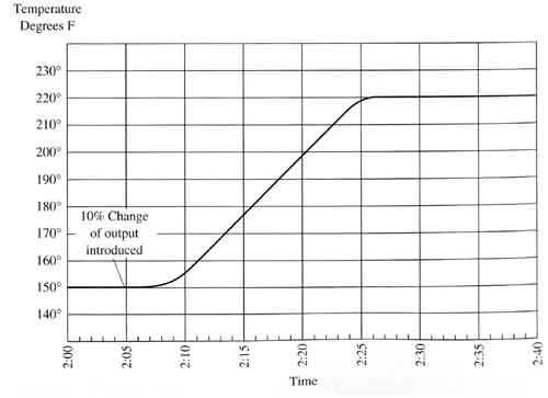
Above: Figure showing temperature (PV) for the barrel of a plastic
injection-molding machine after the output signal is changed a total of
10%.
The next step is to use the graph and determine the amount of process gain, which is the amount of change in the process variable (ΔPV) divided by the amount of percentage change to the output signal from 0-100% (Δ output).
KP = (ΔPV)/(ΔOutput)
(It's important to note that it's the amount of change of these variables and not the actual value that's used in the formula. E.g., if the output signal changed from 40% to 60%, the amount of change is 20%; therefore, the value of 20% would be used in the formula and not 60%.)
KP is called process gain because it will reflect the inherent ability of the barrel to heat up some number of degrees when the output is changed by some percentage.
Don't confuse process gain KP with controller gain KC that has been discussed as "gain" up to now. From the graph in ill. 2 (below) note that the PV was at 150°F when the change was introduced to the output and the temperature increased to 220°F, which is change (Δ) of 70°F. The change (Δ) in the output is 10%. The following formula will show the process gain KP for these values is 7.
KP = (ΔPV)/(ΔOutput)
The next step in this process is to determine the dead time for the system, which is the time it takes for the PV to respond (change) after the output is changed. Dead time is very important since it will be used to determine the amount of integral (reset) response that's needed. The dead time can be found on the graph by locating the point where the output was changed from 10% to 20% and determining how long it took for the PV to start changing. A tangent line is marked on the response graph to show where the change occurs. The bottom end of the tangent line touches the point where the change in PV starts (150°F) when the time is 2:10. The time of 2:10 will be the official point in time where the change begins. Since the 10% change was entered in the system at 2:05 and the system started to change at 2:10, the dead time is 5 minutes.
The third step in the Ziegler-Nichols method is to determine the time constant for the 10% change to the output. The time constant is the amount of time required for PV to change 63% of the total change caused by changing the output 10%. Since PV was 150°F at the start of the change and 220°F at the end of the change, the total change is 70°F, and 63% of 70° is 44°F.
The 44°F change is added to the original temperature of 150°F to determine that the point where 63% change has occurred is 194°F. A vertical line is drawn where 194°F occurs, and you can see it intersects the time axis at 2:18. Since the end of the dead time occurs at 2:10, and the point where the PV is changed 63% occurs at 2:18, the time constant time will officially be determined to be eight minutes (2:18 - 2:10).
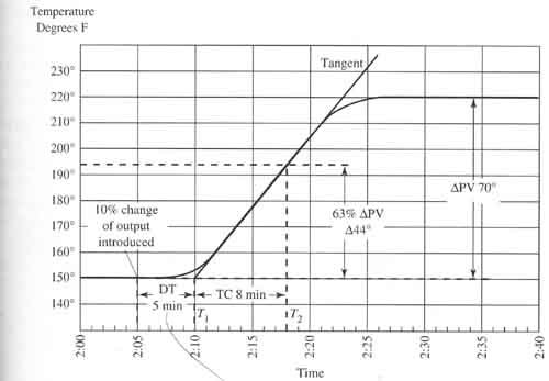
Above: Curve showing PV response that shows the dead time (DT),
time constant (TC), and the process gain (KP) identified.
PREV: Tuning
the Controller
NEXT: Determining PID Values from
Process Gain, Dead Time and Time Constant