AMAZON multi-meters discounts AMAZON oscilloscope discounts
Part II: GENERAL EMC CONCEPTS AND TECHNIQUES
In Part I, the basic techniques necessary for studying EMC were described.
These may be applied to the study of specific problems that affect the EMC behavior of practical systems. A global view of EMC requires a study of the sources of electromagnetic interference (EMI) in the first instance, so that general and specific threats may be identified for each application.
The presence of EMI sources would not be a problem if suitable coupling paths to other circuits were not present. Hence, a study of these paths is necessary and it includes topics such as shielding, apertures, propagation and crosstalk, and coupling at the system level. Finally, the impact of EMI on devices and systems needs to be assessed so that realistic limits and safety margins may be established.
These topics are addressed in Part II using a variety of approaches, including simple intuitive models, analytical formulations, and advanced numerical simulation techniques. The material in the next five sections is particularly relevant to the EMC analyst.
Section 5: Sources of Electromagnetic Interference
The aim of this section is to describe the characteristics of the main sources of EM interference (EMI). The reader will be alerted to the great variety of EM threats and will be introduced to the basic qualitative and quantitative models describing their origin, magnitude, and spectral content.
1. Classification of Electromagnetic Interference Sources
A large number of sources contribute to the electromagnetic environment.
Although in any given application normally only a few of these sources are significant, it is instructive to survey the entire range so that the reader is alerted to various possibilities and is therefore able to ask the right questions when an assessment of EM threats is made. It is undoubtedly difficult to be comprehensive in identifying sources of interference, as each application has its own special features. An astronomical measurement and a domestic electrical appliance are subject to similar EM threats but the dominant design and operational factors are in each case very different. A broad classification of sources of EM interference is useful, however, as it offers a basis for a systematic study. As is natural, the criterion used for classification influences strongly the outcome of this exercise. Sources may be classified according to whether they are continuous or transient in nature. Clearly, in certain applications a transient source of interference may be acceptable, whereas continuous interference would be detrimental to the application. Similarly, sources may be intentional or unintentional in nature. An example of an intentional source is a broadcast radio transmitter, while the radiated interference caused by a computer-to-computer digital signal communication line is clearly unintentional. Another possible classification is into broad- and narrow-band interference. A burst or spike-like disturbance has a broad frequency spectrum unlike, say, interference caused by a mains signal that is at 50 or 60 Hz. A source of interference may be internal or external to a system.
Interference caused by switching operation in a power system is internally generated, but phenomena due to lightning are due to sources external to the system. Many other criteria may be used to classify sources, but in this guide EMI sources are classified into two broad categories, namely, those due to natural phenomena and those due to human activity.
2. Natural Electromagnetic Interference Sources
Human activity, as we understand it, takes place almost exclusively very near the surface of an insignificant planet. It should therefore come as no surprise that this environment is subject to electromagnetic fields that can originate from great distances. We describe these as natural fields.
They are grouped in this section under the heading of low-frequency, lightning, and high-frequency fields.
2.1 Low-Frequency Electric and Magnetic Fields
It may appear at first sight that low-frequency (LF) fields are of no interest to EMC studies. Undoubtedly, coupling to these fields is generally weak except for particular types of instrument. There are, however, some situations where LF fields may cause significant effects. The geomagnetic field is known to all and may be regarded as due to a magnetic dipole with one pole near Antarctica and the other in North America. Both the position of the poles and the strength of the field are subject to variations.
A typical average value is H = 30 A/m. Variations of this field over a period of hours are described as magnetic storms and they generate an associated electric field. It is believed that these storms are related to the sun's activity. Although these fields are small in engineering terms, they may nevertheless cause undesirable effects in large exposed networks.
Varying magnetic fields induce potential differences on the earth's surface (typically 1 to 10 V/km) that can drive current through the neutrals of earthed transformers. Currents as high as 100 A have been measured. The effect of these currents is to drive power and current transformers into saturation, thus causing severe difficulties in the protection arrangements of power systems. Further details, and a description of the effects of a particular geomagnetic storm that occurred on March 13, 1989, may be found in Reference 1.
At a distance of approximately ten earth radii major distortions to the dipole magnetic field are observed (earth's magnetosphere). These are the result of the interaction between particles traveling from the sun (solar wind) and the geomagnetic field.
Under normal fair weather conditions, an electric field of average value of about 100 V/m can be measured at the earth's surface. It is pointing downward, indicating a negatively charged earth. With increasing height the electric field decreases as air becomes more and more ionized. At a height of approximately 50 km, the electrical conductivity is so high as to permit us to describe the earth's surface as the inner electrode of a giant spherical capacitor with the highly ionized layer at approximately 50 km as the outer electrode. The drift of ions between these electrodes contributes under fair weather conditions a total current of about 1500 A to the earth's surface. Clearly, such a situation, if continued, would result in a change to the electric charge balance on the earth. Charge balance is maintained, however, by an opposite current that flows during electrical storms.
A small electric field of the order of a few millivolts per kilometer is also observed in the earth's crust (tellurian electric field). Values depend on latitude, time, and soil properties and increase substantially during magnetic storms.
2.2 Lightning
Lightning is one of the most energetic of all electromagnetic phenomena.
During the lightning phenomenon, the potential difference between earth and thunderclouds is of the order of 100 MV and the charge transfer is of the order of 20 C. Hence, energies of the order of 1010 J are potentially in transit during electrical storms.
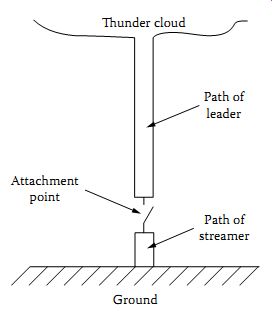
FIG. 1 Schematic of a lightning discharge.
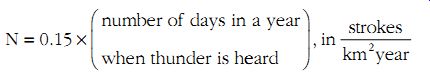
Details of lightning may be found in specialist literature on the subject. A simple phenomenological description of lightning is as follows. Through complex processes, charge separation takes place in thunderclouds so that an excess of negative charge is established near their base. Field enhancement and the resulting ionization result in an ionized channel that proceeds in steps (stepped leader) toward the earth as shown schematically in FIG. 1. As the stepped leader approaches the earth, it causes an upward positive streamer. When the two meet, a highly conducting ionized channel is formed through which a very high current flows (the return stroke). Return stroke currents can be very high. In approximately 10% of all events, the stroke current exceeds 40 kA, and in about 1% of all cases, currents in excess of 100 kA are observed. The current pulse has a rise-time typically 1 µsec and a decay time of 50 µsec. The number of strokes in any locality may be estimated from the following empirical formula
(eqn. 1)
Hence in the United Kingdom, where typically thunder is heard on about 15 days a year, about two strokes per km^2 should be expected in this period. Two types of lightning effects may be distinguished. First, there are direct effects whereby the attachment of lightning to a structure such as a building or aircraft may cause mechanical damage, fires, or explosions.
Second, there are indirect effects whereby the rapid current variations during lightning induce significant interference signals on adjacent circuits and structures. It is this latter case that is of most interest to EMC. Of particular concern is the lightning threat to airborne systems. Measurements on aircraft indicate field values of the order of 600 A/m and 50 kV/m and a rate of rise of current of the order of 150 kA/µsec.
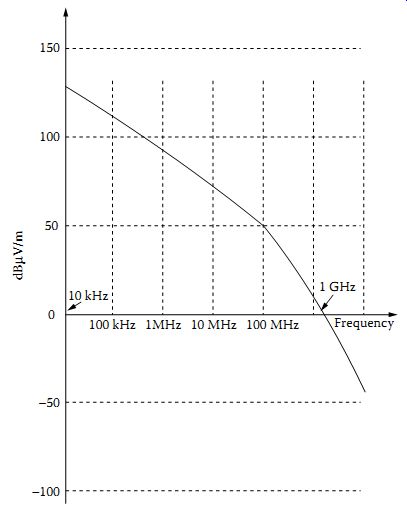
FIG. 2 Amplitude distribution of sferics - peak electric field at
a distance of one mile measured with a bandwidth of 1 kHz.
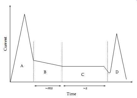
FIG. 3 Idealized aircraft lightning current waveforms (not to scale).
Recent measurements indicate that rise-times as short as a few nanoseconds are not uncommon. Measurements of the spectrum of the electrical field normalized to a distance of 1 mile are shown in FIG. 2.
Comparisons of lightning with other electromagnetic threats [e.g., nuclear electromagnetic pulse (NEMP) and electrostatic discharge (ESD)] may be found in References 10 and 11.
Lightning is a complex and very severe threat, especially for flying systems, with large statistical variations, and therefore arrangements for testing were developed over the years for the lightning certification of aircraft. These are based on idealized current test waveforms, a classification of effects into direct and indirect, and zoning concepts.
The standard test waveform shown in FIG. 3 consists of four components, A representing the initial stroke (peak current 200 kA, action integral 2 × 10^6. A 2s, rise-time 25 µs, and duration 500 µs), B representing an intermediate current (average amplitude 2 kA transferring charge of 10 C), C representing a continuing current (amplitude 100s of amperes, charge transfer 200 C), and D representing a restrike current pulse (current peak 100 kA, action integral 0.25 × 10^6 A2s). The action integral is defined as ? i 2 dt and is a measure of the energy dissipated in resistive parts in the path of lightning (responsible for direct current effects). In contract, indirect effects (e.g., inductive coupling) are dependent on the current and its rate of change. The zoning of aircraft is an attempt to identify parts of its structure most likely to be lightning attachment points. Zone 1 refers to parts with a high probability of attachment (e.g., wing tips, nose, engine nacelle, etc.). Following initial attachment and because of aircraft movement the lightning channel is swept along its surface over areas that constitute Zone 2. Finally all other remaining areas are classed as Zone 3.
International regulations determine which test current waveforms (A, B, etc.) are applicable to each zone.
The increasing use of carbon fiber composites (CFC) in aircraft manufacture because of their strength and low weight has nevertheless enhanced the importance of lightning as a source of interference with aircraft systems (indirect effects) and also direct effects such as rupture of CFC skins, etc. In a nonmetal skinned aircraft the lightning current path is difficult to establish as it may be significantly affected by local features such as fastenings and other conducting structural members. Similarly, indirect effects can be more severe as the EM shielding afforded by the CFC is inferior to that of aluminum. One can see that significant voltage drops appear across the CFC surface that may contribute to common mode voltage on adjacent circuits. Taking the resistivity of CFC as 3500 × 10^-8 ?m and its thickness as 1 mm we obtain its surface resistivity (the ratio of voltage drop per unit length to current per unit width), ?/h = 335 m?/sq.
Hence, a 100-kA peak current will induce a voltage drop of 3500 V/m. The situation will be very different if Al was used (? = 2.8 × 10^-8 ?m).
The EM generated by the lightning channel some distance away may be obtained by considering the channel as an antenna where the current distribution is time and space varying. The current need only be known to obtain the vector potential and then the scalar potential is obtained from the Lorentz gauge condition (see Section 2.2.2). With the two potentials known, the EM field is obtained from Equations 2.34 and 2.35.
2.3 High-Frequency Electromagnetic Fields
High-frequency fields in the range below about 30 MHz are due mainly to terrestrial processes such as electrical storms described earlier and are referred to generally as "static" or "sferics." There are wide seasonal and topographical variations. In general, fields are higher during the night and near the equator, and decrease with frequency. For frequencies higher than about 30 MHz the dominant contribution to the field is extraterrestrial (cosmic) in origin. The earth's magnetosphere, ionosphere, and atmosphere form a partial EM shield to fields originating from outside the earth's environment. At the earth's surface only fields that can penetrate these layers are observed. Penetration is only possible at optical frequencies (infrared to UV) and at radio frequencies between 10 MHz and 37 GHz.
The radio frequency passband of interest to EMC is determined by the shielding properties of the ionosphere and absorption by water molecules.
The sources of cosmic radiation are in the galaxies (strongest near the center) and in the sun. It has been estimated that each galaxy emits about 1035 W in the range 10 MHz to 10 GHz with a large thermal component, but also particular emissions at specific frequencies (e.g., hydrogen at 1.428 GHz). Solar radiation consists of a background level (during a quiet sun), on which are superimposed slow variations (period 27 days), which in the range 1 to 10 GHz may exceed the background value by a factor of three, and radio bursts (flares), which can last from a few seconds to hours with intensities higher by a factor of a thousand compared to background levels.
Due to the statistical nature and wide dependence on location, it is difficult to give specific values for these fields. Surveys of natural back ground radio noise usually quote results in terms of an equivalent or effective antenna noise factor Fa in decibels. Thus, at 10 MHz a typical value for atmospheric noise is Fa = 40 dB, while at 100 MHz galactic noise dominates and contributes approximately 8 dB.
The peak value of the electric field received by a short vertical dipole antenna may be found from Fa using the following formula, which is derived in section E.

(eqn. 2)
where BW is the bandwidth of the receiver in hertz and f is the frequency in megahertz. Further details of the spectral content of natural radio noise are presented in Section 5.4.
3. Man-Made Electromagnetic Interference Sources
The operation of man-made engineering devices makes an increasingly larger contribution to the electromagnetic environment. This may be regarded as a form of pollution and it is expected that increasingly closer attention will be paid to reducing and controlling electromagnetic emissions. A survey of the main sources of man-made EM emissions is given below.
Table 1 Selected U.K. Frequency Allocations [* Different allocations may apply in other regions.]
3.1 Radio Transmitters
This is a form of intentional man-made emission. Mobile and fixed transmitters, radar, and computer-to-computer communications are continuously increasing in numbers, power, and geographical distribution.
International regulatory bodies allocate fixed frequency bands for the different types of application. An example of allocation in the United Kingdom is shown in Table 1.
Clearly, in frequency bands allocated to broadcast transmitters, substantial signal strength may be expected, the EdB V/m F(dB) BW f(MHz) a () log()log . µ= + + - 10 20 95 5
... exact value depending on the power of the transmitter, the distance from the transmitter, and the proximity of other bodies (e.g., buildings, trans mission lines, etc.). Typical urban environment electric field strength due to broadcast transmitters rarely exceeds 200 mV/m. However, near powerful transmitters field strengths of several tens of V/m are possible. Estimates obtained from 250-kW transmitters at a distance of 100 m range from 87 V/m at 4 MHz to 272 V/m at 26 MHz.
Although these emissions are narrowband, interference is also observed at harmonics of the carrier frequency, at sideband frequencies, and there may also be a broadband noise contribution from the various stages inside the transmitter. In a well designed transmitter, harmonics and noise are well below, typically, 70 dB, the strength at the fundamental frequency.
3.2 Electroheat Applications
A valuable means of heating materials is by using high-frequency signals.
In cases where the specimen is highly conducting, heating takes place by inducing currents to it (induction heating), whereas for materials that are poor conductors heating takes place by generating dielectric losses (dielectric heating). Typical frequencies used for induction heating are 1 to 100 KHz, 1 MHz, whereas for dielectric heating, operating frequencies are selected from the following list: 13.560 MHz, 27.12 MHz, 40.68 MHz, 433 MHz, 915 MHz, 2.45 GHz, and 5.8 GHz. Power ratings of several kilowatts are typical. Measurements taken at 30 m away from such heaters have shown average electric field values typically 100 (dB µV/m)18. Harmonics of the operating frequency of domestic microwave ovens have also been investigated as a source of interference at broadcast satellite frequencies (Table 1).
3.3 Digital Signal Processing and Transmission
Modern digital signal processing and transmission methods use fast pulses to code information. Processing, storage, input, and output take place continuously synchronized to an electronic clock. The requirement for higher processing speeds and higher rates of information transfer implies high clock rates and therefore shorter transition times (fall- and rise-times).
Clock rates of several hundreds of megahertz and transition times of a few nanoseconds are common. The presence of fast pulses on printed circuit boards and transfers across communication cables can give rise to radiation and coupling (crosstalk) to adjacent circuits. As indicated in Appendix D, a trapezoidal pulse having a duration t and equal rise- and fall-times tr has an approximately flat spectrum extending up to a frequency 1/pt.
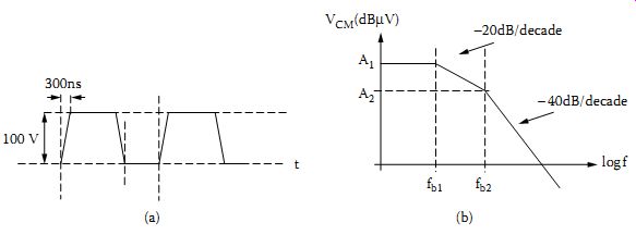
FIG. 4 A pulse in the time-domain (a) and the shape of its frequency
spectrum (b).
Thereafter the spectrum falls by -20 dB/decade up to a frequency 1/ptr.
Beyond this frequency, the spectrum falls by -40 dB/decade. It is therefore evident that substantial power is associated with harmonics of the fundamental frequency and that the highest significant harmonics are determined by the transition time of the pulse waveform. Fast transition times, although desirable from the operation point of view, are undesirable in EMC terms as they make substantial contributions to high-order harmonics. Significant amounts of power are found at harmonics that may be at frequencies twenty times or higher above the fundamental. Estimates of radiated noise for different logic families may be found in Reference 20.
Example: Obtain the envelope of the spectrum for the signal shown in FIG. 4a and then repeat the calculation by changing the transition time to 200 ns. Duty cycle is 50% and f = 50 kHz. Calculate the interference voltage at 3 MHz for the two values of rise-time.
Solution: Following Appendix D, the envelope of the spectrum is as shown in FIG. 4b. We need to calculate the values A1 and A2 and the frequency breakpoints fb1 and fb2. We have....
3.4 Power Conditioning and Transmission
The power supply network is the source and the victim of electromagnetic interference. Although a very high quality of supply is normally maintained, a whole range of signals and disturbances are established on extensive and partially exposed power networks. The presence and the quality of this network, which by its nature is all pervasive, are of great interest to EMC. A broad legal framework exists in most countries, which defines the maximum variation of voltage and frequency (e.g., 240 V ± 6%, 50 Hz ± 1% in the United Kingdom). However, most power utilities maintain a tighter control of their network and impose additional requirements on the quality of the supply. Increasingly, EMC-related regulations impose additional constraints.
A survey of EMC in power systems may be found in Reference 21 and broadly the same classification is used here.
3.4.1 Low-Frequency Conducted Interference
Harmonics - Due to the presence of converter equipment, nonlinear devices such as transformers and arc furnaces24 in power systems, sinusoidal voltages, and currents are generated with frequencies that are multiples (harmonics) of the fundamental mains frequency (50 or 60 Hz).
As an example, a converter contributes signals at harmonic frequencies that are a multiple n of the mains frequency where m = 1, 2, 3, … and p is the converter pulse number p = 6, 12, ….
The voltage total harmonic distortion is defined as
(eqn. 3)
Some of the undesirable effects of harmonics are interference with communications, overheating, maloperation of instrumentation, control and protection systems, and torque pulsations in motors. The level of harmonics varies throughout the day. Of particular concern is the level of the 5th harmonic where values as high as 6% of the nominal voltage have been observed.
Voltage fluctuations - Small changes in the voltage as the result of connection and disconnection of loads are referred to as fluctuations or flicker. The latter term is to indicate the effect that these changes have on the luminosity of incandescent lamps. A 27% fluctuation is considered acceptable provided it does not occur more than once a minute, whereas a fluctuation occurring ten times per minute should not exceed 1.3%.
Voltage dips - Sudden reductions in the supply voltage (more than 10%) followed by recovery within a short time (typically 300 msec) are common in supply networks. Surveys have shown that the causes of these dips and occasional interruptions originate in the medium- and high-voltage networks.
Most of the dips do not exceed 30%. It is estimated that for a consumer in an urban environment, there are about four dips per month that exceed 10% of the nominal voltage. Dips are caused by faults, the switching of large loads, and the starting of induction motors. Dips and interruptions cause problems to data processing equipment and may require restarting and proper sequencing of motors and automatic processes.
Unbalance - The presence of large single-phase loads and the unequal loading of each phase in a three-phase system may cause an in balance in amplitude and/or phase. Some motors may overheat if supplied by an unbalanced source. In practice, unbalance is kept below 2%.
Mains signaling systems - The power network is primarily intended for the transmission of power to consumers. It is nevertheless possible to transmit information that is used for control (public lighting), load management, and tariff fixing. Mains signaling uses relatively high frequencies and networks not specifically intended for signal transmission. There are, therefore, EMC implications, especially since the use of mains signaling is likely to increase in the future. Three types may be distinguished, namely, ripple control systems (100 Hz to 5 KHz, amplitude 5% of the nominal voltage), power-line carrier systems (up to 100 kHz, amplitude 2.5% of the nominal voltage), and home signaling systems used by individual consumers. The EMC implications of using the power network for digital signal transmission are discussed in Reference 28.
Other lower-frequency effects - Voltages may be induced from adjacent circuits, especially during transient conditions, DC components may be present if half-wave rectifiers are used, and small variations in frequency may be present, normally not exceeding 1 Hz/s.
3.4.2 Low-Frequency Radiated Interference
Stray electric and magnetic fields due to power lines and domestic appliances are subject to a variety of limits in various countries. These are normally set with biological effects in mind. At power frequencies electric fields not exceeding 30 kV/m (industrial environment and near power lines) and 0.3 kV/m near domestic appliances may be expected. Magnetic field values rarely exceed 1 mT in industrial environments and 100 µT near domestic appliances and cables.
Much medical apparatus is sensitive to magnetic fields that are a fraction of a micro-tesla and video display units exhibit flicker when the magnetic field is of the order of a few microtesla.
Low-frequency electric fields at harmonics of the power frequency have been studied near 500 kV transmission lines and are reported in Reference 30. Values ranging from 13 mV/m at 15 kHz to 130 µV/m at 200 kHz have been measured. Global measurements of natural background radio noise at power frequencies and contributions made by power lines are reported in References 31 and 32.
3.4.3 High-Frequency Conducted Interference
Voltage spikes in LV networks - A variety of faults and switching operations and lightning strikes on power networks result in a number of spikes (typically ten per day exceeding 200 V) appearing at the domestic consumer level. A number of surveys are available aiming to establish statistical data for spike amplitude and frequency of occurrence. A thorough discussion appears in Reference 33. About 2% of spikes exceed 500 V and about one in a thousand exceeds 3000 V. The duration of most spikes does not exceed a few microseconds, indicating a bandwidth of a few hundred kilohertz. Less than one in a thousand have a duration exceeding 100 µsec. Direct lightning strokes generate overvoltages of the order of 100 kV. These are attenuated as they propagate through the network but surges of several kilovolts in magnitude can be expected at domestic consumer level.
Voltage surges in high-voltage (HV) substations - A substation is a harsh electromagnetic environment, the most severe problems from the EMC point of view being the operation of disconnect switches. With proper control and protection measures, voltage surges do not normally exceed a few thousand volts. A survey of the substation EM environment appears in Reference 34. In modern gas-insulated substations (GIS) where SF6 is used as the insulating medium, faster switching times are obtained with the result that steep-fronted transients with rise-times of the order of 10 to 20 nsec and a rate-of-rise as high as 40 MV/µsec are generated.
These surges, in addition to the insulation problems they cause, also have undesirable EMC effects.
3.4.4 High-Frequency Radiated Interference
Significant radiated fields are measured near substations during switching operations. Electric fields as high as 70 kV/m with frequency components in excess of 200 MHz have been observed. In a conventional substation the data shown in Table 2 are regarded as typical.
Table 2 Radiated Fields Near Substations
Field measurements near a HV DC converter station have been reported in Reference 37. A detailed discussion of EMC in power plants and substations may be found in the CIGRE Guide.
3.5 Switching Transients
Many of the particular examples of interference-generating phenomena, outlined in the last two sections, can be understood by reference to fundamental principles. Many other interference sources, which have not been explicitly mentioned here, can be similarly understood. It is therefore important to present and illustrate these principles in a manner that allows proper characterization of known interference sources and also permits the identification of new ones. This task is tackled in this section.
3.5.1 Nature and Origin of Transients
Although a lot of interference is due to the operation of circuits in steady state, some of the most severe cases of EMI are due to transients that are externally imposed on systems, or those generated internally as a result of normal functional requirements, or in response to abnormal conditions (faults). In an electrical circuit operating under steady-state conditions, energy is stored in particular components such as capacitors and inductors.
Any change in circuit conditions, irrespective of its origin or purpose, requires a redistribution of this energy. Capacitors store energy associated with electric fields.
A capacitor C with a potential difference V across its plates stores an amount of energy given by

(eqn. 4)
Similarly, in a part of space where the electric field is E and the dielectric permittivity is e the energy storage density is (eqn. 5) Inductors store energy associated with the magnetic field and the following formulae apply
(eqn. 6)

(eqn. 7)
Any redistribution of energy in a circuit, whether described by lumped components or more generally distributed components, cannot be done instantaneously. This is a fundamental law of physics, and it implies that during a period of time, however short, potentially large amounts of energy are in transit throughout the circuit. During this period the circuit is described as being under transient conditions. It is important to realize that during this time the values of voltage and current in the different parts of the circuit bear little direct relationship to their steady-state values prior to or after the change. Under these circumstances, overcurrents, over-voltages, and rather fast pulses are not uncommon and these influence EMC behavior decisively.
A qualitative grasp of these phenomena may be achieved by recalling that a capacitor is a component that resists rapid voltage changes. Any attempt to force a high rate of change of voltage (dv/dt) results in a very high current. Similarly, an inductor is a component that resists rapid current changes. Any attempt to force a high rate of change of current (di/dt) results in a very high voltage. Improvements in EMC performance are very often achieved by controlling the rate of change of these quantities under all conceivable (normal and abnormal) conditions. Some examples of how circuits respond to change are given in the next two subsections.
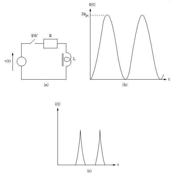
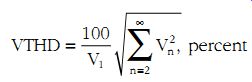
FIG. 5 Closing transient on an inductor (a). Flux (b) and current
(c) waveforms.
3.5.2 Circuit Behavior during Switching Assuming an Idealized Switch
It is perhaps necessary before proceeding further, to state clearly what is meant by an "idealized switch." Let us assume, to start with, that when the switch is conducting (on) it presents zero impedance, whereas when it is not conducting (off) it presents infinite impedance. It is stressed that this behavior is neither available from practical switches, nor, in fact, desirable. This latter point will be demonstrated shortly after a few examples have been studied first. Let us examine what happens when an inductor is connected to an AC source, as shown in FIG. 5a (closing transient in an inductor). It is assumed that the switch is closed at the instant in time when the source voltage has zero value and is rising.
Neglecting the influence of losses (R ? 0) voltage balance in this circuit requires that

(eqn. 8)
...where N and f are the number of turns and the magnetic flux associated with the coil. Integrating this equation gives
(eqn. 9)
where K is a constant.
Assuming that at t = 0 (the moment the switch closes) there was no remanent magnetic flux linked with the coil (f(0) = 0) allows K to be calculated giving

(eqn. 10)
...where fpk = Vpk/(?N) is the peak steady-state magnetic flux in the coil.
This expression is plotted in FIG. 5b and it shows that the maximum excursion of the flux is to 2fpk, twice as large as the value expected under steady-state conditions. In most cases this flux corresponds to a value deep in the saturation region of the material used in the construction of the coil and hence it results in a current that is highly distorted and of a very large peak value, as shown schematically in FIG. 5c. The wave form shown in this figure is rich in harmonics and therefore contributes to EMC problems. The situation is even worse if it cannot be assumed that the remanent flux is negligible. This calculation describes the worst case (losses and a different point-on-wave for switch closure result in a less severe, damped, transient). However, it is not uncommon for the peak magnetizing current of unloaded transformers to exceed, occasionally, twenty times normal values.
A transient of particular interest is that associated with opening an inductive circuit (FIG. 5a). Even for this simple case no progress can be made in obtaining the response of the circuit without some explanation of the properties of the switch. Three possible scenarios are shown in FIG. 6. In each case the switch is opened at time t0 but the subsequent circuit behavior is different.
FIG. 6 Current interruption, abrupt (a), gradual (b), and at the next
current zero (c).
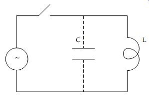
FIG. 7 Opening transient in an inductive circuit.
In case (a) the current I_0 is brought down to zero instantaneously.
Notwithstanding the difficulties of engineering such a switch, it is interesting to speculate what will happen to the energy stored in the inductance just prior to time t0. Clearly, it cannot remain there since there can be no current through L. This is a classic case where the circuit shown in FIG. 3a is not, even approximately, a reasonable model of the physical system. Neglecting losses again for clarity, the model can be improved considerably by adding the "stray" capacitance C shown in FIG. 7. This capacitance could be that associated with the coil, bushing (if the coil is of a substantial high-voltage construction), the switch open contacts, connecting wires, etc. Assuming that the voltage across C is small prior to the switch opening, then at t0 the circuit to the right of the switch consists of an inductor with energy and a capacitor that is approximately uncharged. This circuit will undergo oscillations with a frequency equal to 1/2p . The peak value of the voltage Vpk across the coil and the capacitor can be estimated easily from energy conservation considerations. If losses are neglected, then when the current through the coil is zero, all the energy is stored as electrostatic energy, i.e.,
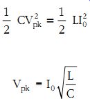
(eqn. 11)
Hence,

(eqn. 12)
Two aspects of this calculation warrant attention. First, the frequency of the oscillations in the L-C circuit is totally unrelated to normal operational specifications, such as the source frequency and, therefore, in principle, a very different oscillation frequency should be expected depending on construction methods and layout (value of C). Second, the magnitude of the peak voltage is totally unrelated to the source voltage.
If the stray capacitance is very small, Vpk can have very large values that may cause flash-over across L and/or sparking across the switch contacts.
In either case there are serious EMC implications.
Let us now examine case (b) in FIG. 6 where the current is brought down more gradually from value I0 at t0 to zero at t1. A linear variation is shown but in practice an exponential decay is normally obtained. Clearly, a switch so designed creates fewer problems for insulation and EMC. The rate of current decay is better defined and can be controlled so that any overvoltages can be kept within specified limits, i.e., V = L ?i/?t where
?t = t1 - t0.
This case is described in more detail in the next subsection.
Finally, a switch may be designed so that in spite of contact separation (tripping) at t0, the current is not effectively interrupted until time t2 corresponding to the next available natural current zero (FIG. 6c).
This is clearly a case where overvoltages are minimized, since no energy is left stored in L to cause further oscillations. In practice it is difficult to achieve interruption exactly at t2 and effectively the situation is not dissimilar to that shown in FIG. 4a, but with I0 being very small. The current at which the switching arc becomes unstable prior to the current zero is known as the chopping current and in a well-designed, high power switch is equal to a few amperes. As an example, the interruption of the HV current in an unloaded 1000 kVA 11/3.3 kV power transformer is studied. The value of L is approximately 14H and C (mainly associated with the HV bushing) is 5000 pF. The "surge impedance" of this coil is therefore Assuming a chopping current of 1.5 A results in a peak voltage 1.5 × 50 × 10^3= 75 kV. This is considerably higher than the operating voltage of this transformer and illustrates the problem of interrupting inductive circuits. When losses are considered and when remanent flux is taken into account the problem appears less severe. For example, if only 50% of the coil energy is recoverable (the remainder is associated with the remanent flux), then Equation 5.12 is modified to give L/C k _ 50-ohm.
V=0.63 I L/C pk 0
The switch characteristic shown in FIG. 6a is not practically achievable, that shown in FIG. 6b is typical of switching at low voltages (e.g., fuses), and the characteristic shown in FIG. 6c is typical of high-power circuit breakers.
Let us now examine the case of the opening transient in a capacitive circuit. A typical circuit is shown in FIG. 8a. It is assumed that the current is cleared at a natural current zero (t0) as shown in FIG. 8b.
The source voltage VA is also shown and it is clear that for t > t0 the potential of point B remains constant at -Vpk. The potential difference across the switch is therefore Vsw = VA - VB as shown in FIG. 8b. The maximum excursion of Vsw is to 2Vpk, thus causing substantial stress on the insulation of the switch. Should the switch fail under these circum stances and reignite, thus re-establishing conduction, fast oscillations will occur with any circuit inductance, as was the case for the inductive transient described earlier, but now with the initial energy store provided by the capacitor. Again, as before, there are important implications for EMC.
All the transients described above were studied using lumped circuit components. The situation is similar in principle, but considerably more complicated, when distributed parameter circuits are involved. For example, interrupting the charging current of an unloaded transmission line is similar to opening a capacitive circuit but with the added complication of the presence of traveling waves and reflections. Further information on transients and parameter values for transient calculations may be found in Reference 39.
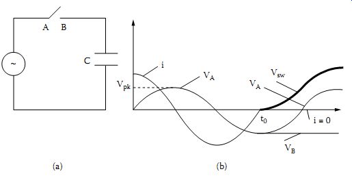
FIG. 8 Opening transient in a capacitive circuit (a). The voltage
across the switch Vsw = VA - VB is shown in heavy outline in (b).
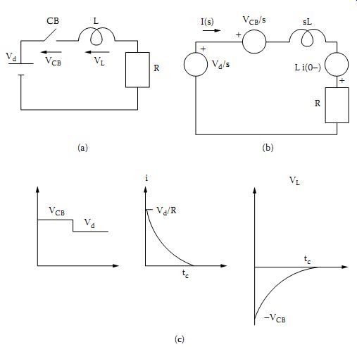
FIG. 9 Influence of arcing voltage on current interruption (a). The
breaker voltage, current, and voltage drop across L are shown in (c).
3.5.3 Circuit Behavior during Switching Assuming a Realistic Model of the Switch
Switching elements, whether of the solid-state type or electromechanical, exhibit complex behavior. In most cases the user of such components has a limited grasp of their full operational features and even the specialist is hindered by the lack of well-documented, easily accessible information essential for modeling such components. Switch behavior is crucial in EMC studies. Three domains are important in the operation of a switch.
First, switch behavior prior to actual current clearance; second, behavior around the point when the current is cleared; and third, its behavior after current clearance as it fully recovers its dielectric strength.
Let us first examine how current is cleared in a low-voltage circuit.
The DC circuit shown in FIG. 9a is studied. It is assumed that initially CB is closed and that steady-state conditions have been established. The electromechanical circuit breaker CB is tripped at t = 0 and it is assumed that the voltage drop across the arc is equal to VCB and remains constant until the current is brought to zero. The time taken to clear this circuit is required together with the voltage VL across the inductor. The circuit may be solved using Laplace transforms with the operational equivalent shown in FIG. 9b. The Laplace transform of the current is found to be
Using tables, the current following the opening of the switch is found to be....
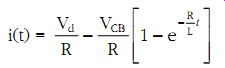
(eqn. 13)
The time it takes to force the current to zero is obtained from this expression and is....
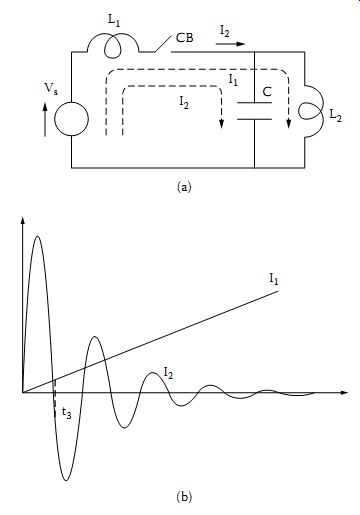
FIG. 10 Circuit used to study arc re-ignition (a) and current components
at power and high frequencies (b).
The voltage across the inductor is....
The waveforms for VCB, i, and VL are sketched in FIG. 9c. Clearly, the arcing voltage must be higher than Vd to effect current clearance. If VCB=1.1 Vd then tc_ 2.4 (L/R). The magnitude and duration of the inductive voltage drop are crucially dependent on the arcing voltage. In practice the behavior of the switch during arcing is considerably more complex, but the simple calculation above illustrates the essential features of switching.
Let us now examine in more detail how a practical electromechanical switch may behave following current interruption. A typical circuit that illustrates the essential parties to this phenomenon is shown in FIG. 10. Following the parting of the contacts, the current ICB through the switch consists of two parts. First, there is component I1, which is due to the power source. In the short time after interruption of interest to this study, the source voltage may be considered to remain approximately constant, at its value at the moment of interruption Vs(0). Hence I1 is approximately equal to Vs(0)t/(L1 + L2). Second, there will be a high frequency component I2, which is oscillatory in nature and is due to the redistribution of energy trapped in the energy storage circuit elements.
The frequency of this component is very high compared with that of the source. Both components are sketched in FIG. 10b. It is clear that there are moments, such as t3, when the switch current Isw is equal to zero. The voltage VCB, which appears across the switch, is similarly affected by high-frequency voltages. Following contact separation at t0 and current clearance, say, at t1, the circuit breaker recovers its dielectric strength relatively rapidly. The breaker recovery voltage shown by a broken line in FIG. 11a illustrates this recovery. Following current interruption at t1 a transient voltage appears across the breaker, as shown schematically by curve AB. At time t2, the voltage applied to the breaker is about to exceed the level that can be sustained across the contacts. The breaker then reignites and conduction is reestablished. The breaker circuit is now made up of components I1 and I2 as explained earlier, and goes through zero at time t3 as shown in FIG. 11b. At this point the breaker may be able to clear the current again. The transient voltage difference across the breaker will then increase as shown by CD in FIG. 11a. Another reignition is likely at time t4 with a further current clearance at t5. This process may be repeated several times until the breaker has recovered sufficiently to sustain the maximum applied transient voltage. The phenomenon just described is referred to in the literature as "showering arc" and it is capable of producing EMI in the megahertz range.
Another manifestation of the same phenomenon, but without the involvement of a circuit breaker, is the so-called "arcing ground." This is particularly important in ungrounded systems where a fault to ground combines with high-frequency transients involving capacitances to earth to produce a series of fault arc extinctions and re-ignitions.
=======
Table 3 Triboelectric Series
Positive charging Air
Hands Glass Mica Nylon Wool Aluminum Paper Steel Acetate Polyester
Polypropelene
Pvc Negative charging
Teflon
========
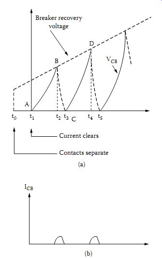
FIG. 11 Breaker recovery and re-ignition (a) and breaker current (b).
3.6 The Electrostatic Discharge (ESD) Large material bodies are to a high degree electrically neutral. However, charge separation and charging can take place when two bodies, of which at least one is insulating, come into contact and subsequently separate.
This is known as the triboelectric effect and it is one of the oldest known of electrical phenomena.
Some materials have a propensity to acquire electrons on contact, whereas others give away electrons easily. The former tend to charge negatively, whereas the latter tend to acquire positive charge.
Materials may be placed in a triboelectric series according to their tendency to charge positively or negatively. An example is shown in Table 3.
Charging may also occur by induction whereby a charged body A causes charge separation in a neutral body B. Temporary grounding of B causes some of its charge to leak away, thus leaving B charged. The typical process involved is the charging of an insulator and the subsequent discharge (ESD) through a conductor to another conductor, which may be grounded. The most common problem is that of the charging of humans brought about by walking on low electrical conductivity materials (carpets).
It has been found that the human body can charge to a potential often exceeding 10 kV. A phenomenological description of ESD in this case is as follows: Due to the triboelectric effect the shoes are left with negative charge. By induction, charge separation takes place in the body so that the lower extremities are positively charged and the upper body extremities are negatively charged. On approaching another body, an intense electric field is established that may result in an ESD. It has been found that the discharge has a shorter rise-time for faster approach and for lower voltage.
An approximate equivalent circuit is shown in FIG. 12a. Component Cb represents the body capacitance to ground (typically 150 pF) and Rb the body resistance (typically 1.5 k?). Due to triboelectric effects Cb may be charged to several kilovolts. When A is brought into contact with a grounded conducting body, the capacitor discharges, thus causing the flow of current, which results in conducted and radiated interference. An improved model is shown in FIG. 12b where a small inductance Lb has been added and branch B-C is a model of the human hand. The discharge current has a fast rise-time component (less than 1 nsec) due to branch B-C and a slower component (100 nsec) due to branch B-G.
Peak currents of several tens of amperes are typical. Measurements and analytical results of radiated fields due to ESD were reported in Reference 49.
An electric field value of 75 V/m was measured at a distance of 1.5 m from a 2-kV ESD. Electrostatic charging problems are also observed in airborne systems, e.g., satellites.
The fast rise-time pulses due to ESD may interfere with clock transitions in digital circuits and thus cause upsets and malfunctions.
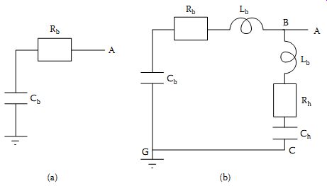
FIG. 12 Simple (a) and more complete (b) equivalent circuit used to
study ESD from the human body.
3.7 The Nuclear Electromagnetic Pulse (NEMP) and High Power Electromagnetics (HPEM)
A high-power electromagnetic pulse (NEMP) is produced following a nuclear detonation. The basic phenomenology is as follows: Following a nuclear detonation a large number of photons (?-rays) are produced and spread through space. These photons interact with the surrounding material to produce high-energy electrons (Compton effect). The Compton electrons travel at high speed and are thus the source current producing intense electromagnetic fields. These electrons produce further, secondary, electrons that increase the conductivity of the surrounding medium. The temporal and spatial development of the NEMP are therefore very complex as they involve the interaction of high-energy particles with materials.
Other effects, such as those due to interaction of neutrons, and distortions in charged particle trajectories due to the earth's magnetic field contribute further to this complexity. More details may be found in References 51 and 52. Three types of NEMP may be distinguished. First, explosions at high altitudes (>100 km) described as high-altitude EMP (HEMP); second, explosions near the ground; and third, system-generated EMP (SGEMP).
The distinctive feature of HEMP is that it affects a very large geographical area and thus presents a simultaneous threat to a large number of systems. Although waveform details are classified, EMP studies are done using a standard NATO pulse to describe the electric field of a H_EMP.
The form of this field is (eqn. 14).
This pulse has a rise-time of a few nanoseconds and a decay time of less than 1 µs. The peak electric field is of the order of 50 kV/m. The energy flux associated with this field is of the order of 1 J/m2 and therefore represents a significant threat. A slower, less severe field lasting for hundreds of seconds follows this sharp pulse (magnetohydrodynamic EMP). Extensive exposed systems, such as power transmission networks, are particularly vulnerable to HEMP. Currents may be induced into these systems causing effects similar to those due to geomagnetic storms (protection malfunctions, transformer saturation, etc.).
Surface EMP refers to explosions near the ground and the associated EM effects have a much more limited geographical range than HEMP.
Inevitably, studies of surface bursts involve ground effects and are almost always near the source (SREMP). Such studies are therefore particularly difficult and there are no guidelines regarding standard waveforms suitable for equipment hardening tests.
Finally, SGEMP involves the interaction of incident particles and pho tons with equipment casings, etc., thus producing very high fields and damage to electronic components.
The strategic objective of NEMP studies is to harden and thus maintain the integrity of critical paths and equipment, so that decision time is increased and enough capability survives a first strike to offer a credible deterrent.
Comparisons of the threat to systems posed by NEMP and by lightning (LEMP) may be found in References 10 and 11.
There is considerable interest in studying Intentional Electromagnetic Environments (IEME) that may result from hostile action or terrorism. A number of experimental systems were developed to evaluate impact.
Narrow-band systems can deliver hundreds of megawatts of power in the frequency range 1 to 3 GHz. Moderate band systems delivering power in the range 100 to 700 MHz are also available. Broadband systems such as JOLT53 can deliver a 100-ps pulse with a field-range product rEpk _ 5.3 MV.
The bandwidth of this system covers the range 40 MHz to 4 GHz. A survey of specialized HEMP systems may be found in Reference 54.
4. Surveys of the Electromagnetic Environment
Various organizations provide data characterizing the electromagnetic environment in specific areas or in general terms. A useful collection of survey results relating to mains transients may be found in Reference 33.
Large surveys of radio noise are prepared by the International Tele communication Union (ITU). Data for external noise levels in the range 0.1 Hz to 100 GHz are reported in Reference 55. In broad terms, the external noise figure in decibels ranges from a value of 260 at 1 Hz to a value of 150 at 1 kHz. More details and values at higher frequencies may be found in the report quoted above. Important also is a survey by the ITU on man-made radio noise.
This report gives the mean value of noise power in decibels above thermal noise at 288 K, in the form where f is in megahertz and the coefficients c and d depend on the actual environment. As an example, in a residential environment c = 72.5 and d = 27.7. Further details may be found in the report quoted above. Similar information is provided in standards concerned with the establishment of EMC limits.
In many cases, a systematic electromagnetic survey is necessary to establish the amplitude, frequencies, timing, and spatial details of electro magnetic signals on a particular site. This information is used to study the influence of EMI on equipment installed on this site.
Prev. | Next