Measurement of Noise

Sound and noise are simply pressure waves traveling through the air at the speed of sound (1122 ft/sec or 765 mph) under standard atmosphere conditions. (Sound waves can also travel through other media at higher velocities, but that's outside the subject of transducers.) It logically follows that to measure sound it's only necessary to measure the pressure of the wave(s) caused, using a suitable transducer .

The actual physical pressures involved are quite small but ex tend over a considerable range. Sound pressure levels are expressed in decibels (dB), the significance of which will be explained later. The actual pressure produced by any sound pressure level is then given by

pressure (lb/in.^2) = 29 x 10^dB/20 x 10^-10

For example, 80 dB is a fairly loud sound. Calculating the equivalent pressure, we get

pressure = 29 x 10^80/20 x 10^-10

= 29 x 10^4 x 10^-10

= 0.000029 lb/in

We need a very sensitive transducer to respond to such low pressure levels and connect it into a measurable/undetectable quantity (for example, a meter reading). Fortunately, we have one in the microphone. Microphones are, in fact, the standard form of transducer used for measurement of sound.

Now to return to the subject of decibels. A human being (and presumably also animals, birds, and other creatures) detect sound as an energy intensity level. The lowest sound intensity level that can be detected by the average individual is 10^-12 W/m^2. This level is described as the threshold of hearing

With increasing intensity levels, sound appears louder and louder, until eventually the sensation received changes from hearing to feeling. This occurs at a sound intensity level of about 1 W/m and represents the threshold of feeling

The intensity or sound energy range covered between just hearing and the threshold of feeling is thus from 10^-12 to 1, or a range of 1 million million. Such a simple linear scale is far too large to work with, so we use one related to the ratio of intensity levels, called bels, and expressed by the formula

bels = log10 (I_h/I_o)

where Ih is the sound intensity level of the sound heard

I_o is the sound intensity level at the threshold of hearing

Even this proved too broad a scale, so a smaller unit of one- tenth of a bel, called a decibel, is used: thus,

decibels (dB) = 10 log10 (I_h/I_o)

This gives a range of 120 dB between the threshold of audibility and the threshold of feeling. It also establishes a useful figure to remember: a doubling in sound intensity corresponds (almost exactly) to a rise of 3 dB.

This can be proved as follows. If I represents the original sound intensity, and 12 the doubled sound intensity, the dB relationship is

dB = 10 log10 (I₂/I₁)

= 10 log10 (2I₁/I₁)

= 10 log10 (2/I₁)

= 10 log10 (2/I₁)

= 3.01

This is not the complete story, especially concerning sound transducers. They detect sound pressure level. Now sound intensity is proportional to the square of the corresponding sound pressure level, so the dB relationship for sound pressure levels becomes

dB = 20 log10 (P₂/P₁)

In other words, doubling the sound pressure level is equivalent to a rise of 6 dB.

Thus because sound is measured in terms of sound pressure level, a change of 6 dB represents a doubling or halving of sound intensity as distinguished by the human ear.

BASIC SOUND MEASUREMENT TECHNIQUE

A microphone converts sound pressure impinging on it into an electrical signal that can be amplified as necessary to provide a readout. However, the transducer signal output will normally be a ragged ac-type signal alternating rapidly from positive to negative levels, which is impossible to display except on an oscilloscope. To obtain a meaningful readout for instrumentation, therefore, you must interface the transducer with circuitry that modifies the out put signal so that both positive and negative parts are rendered as a positive signal, although varying in amplitude at audio frequencies. For a steady “average” reading the signal is put through a time constant circuit; the square root of the average signal is then extracted to give a root-mean-square (rms) average reading.

In the practical sound-level meter the time constant circuit normally provides two averaging time constants: one slow (about 0.9 sec), and one fast (about 0.125 sec). Slow speed is selected for measuring fluctuating sounds; fast speed is selected for measuring continuous, reasonably steady noise. If in doubt as to the character of the noise, you can measure it on both settings and com pare them. If the fluctuations in meter reading on fast-setting range are less than 6 dB, then the average reading should agree with the reading attained on slow setting.

In addition, the sound-level meter incorporates a calibrated alternator network, enabling reading range to be switched to various levels (usually in 10-dB steps). This basically is equivalent to ex tending the length of scale of the meter reading by the number of alternative steps provided.

WEIGHTING NETWORKS

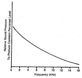
Fig. 22-1. Relative sound pressure required to produce a given perceived level of sound as a function of frequency.

Averaged sound pressure levels read as a single number indicated on a meter still have one basic limitation. They are a purely quantitative measurement of sound, which differs from subjective response to sound level at different frequencies (see Fig. 22-1). Here the curves correspond to different “loudness levels,” as heard, showing how apparent loudness changes with frequency. It will be seen that at lower frequencies lower sound pressure levels give the same apparent loudness. Thus, low-frequency sounds appear to be “louder” than higher-frequency sounds at the same sound pressure level. (High-frequency sounds can be more disturbing, however.)

To overcome this, we add a weighting network to the meter circuit, which has the effect of adjusting the final averaged signal out put to compensate for this effect (Fig. 22-2). The usual form of employment is A weighting, when the corresponding scale readout is calibrated in dB(A). This is now universally employed for single- number noise measurement and is generally in close agreement with subjective ratings. Meters may also incorporate other weights, such as B, C, and D, but those are used for more specialized purposes.

Fig. 22-2. An approximate graph of relative gain versus frequency for an equalizing circuit, designed so that the human ear perceives sound intensity according to the actual sound pressure.

The single-number reading dB(A) sound-level meter is a relatively simple instrument, easy to use and understand, and generally suitable for comparative purposes. It still has many limitations, however. It is measuring only a (weighted) average sound pressure level that gives no indication of the active frequency content of the sound. More complex instruments employ additional filters and circuitry to measure sound pressure levels at different frequencies, which enables the actual distribution of sound content to be analyzed; from this a frequency spectrum can be plotted or presented on a display. This is concerned entirely with electronic circuitry and is outside the subject of transducers. The transducer (microphone) provides the original signal information only. To what degree it's amplified, averaged, weighted, alternated, and analyzed depends on the following electronic circuitry and readout system adopted.

MICROPHONES

Microphones are the only transducer involved in noise- measuring instruments. The two main types are piezoelectric and condenser. Piezoelectric microphones employ a crystal of piezoelectric material as a transducer. They may also be known as c or ceramic microphones. Condenser microphones, also known as electrostatic or capacitor microphones, work on the principle of variations in electrical capacitance to provide an output signal. They are generally more prone to self-noise and require more extensive instrumentation than ceramic types, but they can offer advantages for specific applications—for example, when good high-frequency characteristics are required.

Other types of microphones that may be used include moving- coil or dynamic types and special directional microphones, which may incorporate any one of the three types of elements. Dynamic microphones are, however, relatively limited in application and have the basic disadvantage that comparatively large sizes are necessary to avoid distortion at low frequencies.

Hydrophones are a further type of microphone, designed specifically for underwater sound measurement. They normally employ piezoelectric elements.

Table 22-1 gives a general comparison of different types.

The choice of microphone depends on a number of factors. Low self-noise is obviously desirable, for example; for a microphone used to measure low sound levels, this is essential. The ceramic type is the preferred choice in this case, because even under the best conditions the inherent self-noise of condenser-type microphones can seldom be reduced below about 20 dB. A further requirement for the measurement of low sound levels is that the output voltage generated by the microphone must override the circuit noise of the amplifier in the sound-level meter.

The measurement of high sound levels requires that the system be free from microphonics or spurious signals generated by vibration. This is generated in the circuit components rather than the microphone, but mechanical vibration can also affect the microphone itself. A relatively soft type of mounting and special types of low-sensitivity microphones for measurement of very high sound levels may be required.

Microphonics are not normally experienced, except where sound pressure levels in excess of 100 dB are being measured, unless the microphone or instrument is mounted in such a way that mechanical vibrations are transmitted directly to it.

Both the piezoelectric and condenser microphones are generally well suited for the measurement of low-frequency noise, although moving-coil types can have distinct limitations imposed by their physical size. Accurate measurement of high-frequency sounds calls for the use of a small-size microphone. Regarding frequency response, the condenser type offers a narrower deviation range and the possibility of extending accurate measurements up to frequencies of 20,000 Hz. Both types can, of course, be calibrated for correction. Special types of microphones are required for accurate measurement of frequencies in excess of 20,000 Hz, or above the audio-frequency range.

The final choice of type can also be affected by humidity and temperature. A number of piezoelectric crystals, for example, are sensitive to humidity and can even be damaged if humidity is too high. In unfavorable ambients the piezoelectric element must therefore be rated as suitable for working at the prevailing humidity and /or temperature.

Condenser microphones are also sensitive to humidity, although they are not necessarily damaged by high humidity. Sensitivity, in this case, is caused by electrical leakage across the microphone, which tends to increase with increasing humidity. Exposed insulating surfaces are generally treated to maintain low leakage with high humidity, but it's not necessarily positive protection under all conditions. Some authorities recommend that the microphone be kept at a higher-than-ambient temperature to reduce leakage.

Other microphones have much higher maximum service temperatures. Condenser microphones normally have a maximum service temperature of the order of 100°C. In the case of portable instruments, temperature limitations are normally restricted to battery performance. Battery life will tend to be shortened at temperatures in excess of about 500 C., and battery output may be insufficient at near-zero or subzero temperatures, depending on battery type. Special batteries are required for satisfactory operation at subzero temperatures.

All microphones are temperature sensitive. Calibration is carried out at a normal ambient temperature, and sensitivity will vary at different temperatures. This is generally negligible in the case of piezoelectric microphones, where the temperature coefficient is only of the order of -0.01 dB per degree Celsius. With a typical condenser microphone the temperature coefficient can be as much as four times greater.

Fig. 22-2. An approximate graph of relative gain versus frequency for an equalizing circuit, designed so that the human ear perceives sound intensity according to the actual sound pressure.

MICROPHONE CALIBRATION

Microphones for sound-level meters are calibrated by the manufacturers with microphone reciprocity calibrators, whereas sound-level calibrators are used for overall calibration of sound-level meters. Acoustic calibrators can provide an overall calibration check in field use, but not necessarily with original accuracy. Many meters have built-in electrical calibration and internal calibration controls that enable electrical calibration to be carried out, but this is only a check on the stability of the electrical system.

The following comments largely cover the question of calibration as far as the average user of sound-level meters is concerned:

- Initial (manufacturer’s) calibration of the instrument can usually be regarded as adequate for about a year, after which a calibration check should be made. Such calibration is normally based on free-field response to noise of random incidence. The accuracy given by the calibrated meter then depends on the stability of the microphone and stability of the electrical system; the validity of the measurement is dependent on the characteristics of the sound field present when the measurement is taken.

- Electrical calibration is a useful check on the stability of the electrical system of the calibrator and can be carried out quite simply at regular intervals, such as monthly (especially if meters have built-in electrical calibration and internal calibration controls).

- The use of an additional (calibrated) microphone can pro vide a simple comparative check as to whether the original microphone has changed in characteristics and thus needs calibration. This method, used with electrical calibration, provides the simplest overall calibration check. Note, however, that this depends on the second microphone being used only for checking and being carefully stored.

- Acoustic calibrators can provide an overall calibration check under “field” conditions, but the accuracy of such a calibration check depends both on the suitability of the instrument and its proper method of employment (particularly regarding sealing of the microphone in the sound chamber).

- An exact calibration check can only be carried out under laboratory conditions. It is generally recommended that instruments be returned to the manufacturer(s) at suitable intervals (about once a year) for such a check.

- Calibration should always be checked if the instrument is subject to shock, such as being dropped or receiving rough handling.

USING SOUND-LEVEL METERS

Most people using sound-level meters adopt a “point-and-read” technique. This is generally (but not completely) satisfactory when sound levels are being measured in a large open area (for example, outdoors), or under free-field conditions. This broadly implies that there are no surfaces present to produce sound reflection at the point where the measurement is being taken. Most meter microphones are omni-directional and thus pick up sounds coming from all directions.

Wind blowing directly onto the microphone can produce false readings, although this effect is minimized when the microphone itself is fitted with a windshield. Note also that wind can affect the strength of noise measured from a distant source, depending on wind strength and direction and the distance from the source. The same noise source will give a higher reading downwind than up wind at the same distance from the source, for example.

Although most microphones used for sound measurement are omni-directional, this may only apply as far as low-frequency sounds are carried. At higher frequencies, where the wavelength of the sound may be comparable to the size of the microphone itself, considerable directional effect may be present. In this case the measured response will vary with the direction in which the microphone is pointed.

As a general rule, for accurate measurement a sound-level meter should be held at arm’s length sideways with the microphone pointed away from the noise source, i.e., with the sound impinging on the microphone at grazing incidence (90 deg). However, this will depend on the type of microphone. Some may need to be pointed directly at the noise source for free-field measurement. Requirements in this respect will be specified in the manufacturer’s instructions. Errors as large as ±6 dB may occur through bad positioning of a hand-held sound-level meter, due mainly to the presence of the operator. For most accurate results the meter (or separate microphone) should be clamped in position, and operator and any other instrumentation moved a short distance away.

MEASURING INDOOR NOISE

Accurate measurement of noise levels in rooms or buildings is complicated by the fact that sound reflections are inevitably present, the strength of which will vary at different points. Thus, the actual position at which the reading is taken is significant. Also if the noise generated by a particular source is being measured (for example, a machine), the meter records not only machine noise but background noise as well.

To complicate the question still further, the behavior of noise in the near field differs from that in the far field; it's also affected by the shape of the noise field.

Here “field” refers to the hemispherical distance of the point of measurement from the source—call this R—or the radius of the hemisphere, which is simply the linear distance between noise source and the point considered.

Normally sound level decreases according to distance squared, i.e., by I/R^2. In the near field, or for small distances (small values of R), sound intensity will decrease at a lower rate than given by this law. At some value of R, propagation of sound-level intensity then changes to follow the inverse-square law, or the condition changes from near field to far field.

Measurements made in the near field would, therefore, give a false value if extrapolated on the noise-law basis to estimate such level at a greater distance. Similarly, measurements taken in the far field would give a false (low) rate if used to estimate noise level at a short distance from the noise source in the near field.

The point at which the near field changes to the far field depends both on the bulk and shape of the noise source and on whether noise is emitted uniformly from that shape. If we assume that the latter applies, then the extent of the far field can be estimated as being at least three times, and no more than five times, the linear dimension of the noise source “facing” the point considered. Taking measurements at a greater distance than this should ensure a true far field reading when the noise law applies for any 5 recalculations or estimates required.

Note, however, that most practical noise sources have both bulk and non-uniform radiation of sound. In other words, they are directional noise sources, radiating sound more in some directions than others. This can only be discovered by taking measurements at various positions around the source and , if necessary, plotting equal sound-level contours.

In general, sources of low-frequency noise tend to be non-directional (uniformly radiated), particularly when the source itself is small in comparison with the wavelength of the sound being generated. Directional effects tend to become more apparent as the sound frequency increases, particularly when the source of the sound becomes large in comparison with the wavelength of the sound.

REVERBERANT FIELD

In a room the walls, ceiling, and floor all form reflecting surfaces. If we assume a point source of sound, the sound field within the room has two components:

- The direct sound SD between the source (S) and receiver (R) (Fig. 22-3A). This is the same as free-field conditions and is not modified by the presence of the enclosure.

- The reflected sound SR, which reaches the receiver after one or more reflections from the enclosure surfaces (Fig. 22-3B). The value of this is determined by the power of the source and the reflecting properties of the enclosure surfaces. With perfect reflection the value of SR would eventually rise to extreme values, regardless of the value of the source. In practice, this is impossible, but nevertheless the combined value of SD and SR can give rise to very high levels at any point R with highly reflective enclosure surfaces. Marked variations in sound pressure level at different points R will also be experienced due to interference effects between the multidirectional waves. This will be further modified by a non-point source.

If the size of the source is small relative to the dimensions of the room, there will be a definite distinction between the effects of the direct sound and the combination of direct and reflected

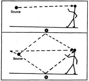
Fig. 22-3. At A, direct propagation of sound; at B, reflected propagation.

SEMIREVERBERANT FIELD

sounds. Near to the source, direct sound will predominate, and the effect of reflected sound components will tend to be negligible. At some greater distances, reflected sound will predominate: the region in which this occurs is known as the reverberant field. The inner boundaries of this field will be determined by the size of the room, the absorption characteristics of the reflecting surfaces in the room, and the acoustic power, size, and directivity characteristics of the source.

Fluctuations in sound pressure levels in the reverberant field due to “interference” effects yield patterns that are known as standing waves. In general, these are most marked when the source has frequency components corresponding to, or close to, any of the possible resonances of the room. The spacing of such standing waves tends to be slightly greater than one-half of the wavelength concerned.

In practice, in most rooms in which sound measurements are semi-reverberant: the walls, ceiling, and floor are neither completely reflecting nor completely absorbent. If sound measurements are made in such a room in the same way as in a free field, correction is necessary to obtain equivalent free-field sound pressure level readings. This necessitates evaluation of the room characteristics or room constant. Rooms with a large degree of absorption have a large room constant and approach free-field conditions. Rooms with a large degree of reflection and only a small degree of absorption have a low room constant and approach reverberant-field conditions.

The main constant can be expressed in terms of the ratio of sound decay in the room (D). This is normally determined as reverberation time or the time in seconds required for the sound pressure level to fall to 60 dB when the source is shut off. The decay rate then follows as

D= 60 / reverberation time

Once the decay rate has been established or estimated, the average sound level in that part of the room where the reverberant field applies can be estimated from the equation

SPL = PWL - 10 log10 V - 10 log10 D + 48

where PWL is the source power level

V is the volume of the room in cubic feet

D is the decay rate, as defined above.

It should be noted that this formula gives approximate answers only. Correction may also be needed to compensate for changes in atmospheric pressure, temperature, and relative humidity.

BACKGROUND NOISE

The question of background noise causing inflated readings when measuring the noise of some individual source is normally not too significant. Take a reading with the noise source switched off. This is the background noise. Now take a reading with the noise source switched on. This is a “combined” reading of the noise source and background noise level. However, if the difference between the two readings you have taken is 6 dB or more, then the effect of the background can be ignored entirely.

Suppose, for example, the background noise level measured was 55 dB. With the noise source switched on the new reading is 65 dB. This is a 10-dB difference, so certainly the combination of the background noise can be ignored. It is only when two nearly equal sound sources are present at the same time that the lower one has any appreciable contribution to noise level measured.

Here, however, we must be careful. The combined sound level of two near-equal noise sources is not the arithmetical sum of the two dB values. The amount added to the overall noise level is related to the difference between the two. This is somewhat complicated to work out mathematically, but Table 22-2 gives satisfactory answers. For differences greater than 6 dB the amount to be added becomes negligible.

Table 22-2. Combining Near-Equal Noise Levels

Example 1. Find the combined sound level of two equal sound sources, each of 55 dB.

difference = 0

so amount to be added is 3 dB

Combined sound level = 55 + 3 = 58 dB

Example 2. Sound level A is 68 dB, and sound level B is 71 dB.

Find the combined sound level.

difference = 3 dB

so amount to be added to loudest (B) is 1.75 dB.

Note. In practice, sound levels are never quoted in decimal fractions values are rounded up or down to the nearest whole number.