AMAZON multi-meters discounts AMAZON oscilloscope discounts
1. Introduction
The different forms of motion have already been explained in the introduction to the last SECTION. In that introduction, it was explained that motion occurred in two forms. These are translational motion, which describes the movement of a body along a single axis, and rotational motion, which describes the motion of a body about a single axis. Because the number of sensors involved in motion measurement is quite large, the review of them is divided into two SECTIONs. The last SECTION described translational motion sensors and now this SECTION describes rotational motion sensors. Again, as for translational motion, rotational motion can occur in the form of displacement, velocity, or acceleration, which are considered separately in the following sections.
2. Rotational Displacement
Rotational displacement transducers measure the angular motion of a body about some rotation axis. They are important not only for measuring the rotation of bodies such as shafts, but also as a part of systems that measure translational displacement by converting the translational motion to a rotary form. The various devices available for measuring rotational displacements are presented here, and arguments for choosing a particular form in any given measurement situation are considered at the end of the SECTION.
2.1 Circular and Helical Potentiometers
The circular potentiometer is the least expensive device available for measuring rotational displacements. It works on almost exactly the same principles as the translational motion potentiometer except that the track is bent round into a circular shape. The measurement range of individual devices varies from 0-10 deg to 0-360 deg depending on whether the track forms a full circle or only part of a circle. Where a greater measurement range than 0-360 deg. is required, a helical potentiometer is used. The helical potentiometer accommodates multiple turns of the track by forming the track into a helix shape, and some devices are able to measure up to 60 full revolutions. Unfortunately, the greater mechanical complexity of a helical potentiometer makes the device significantly more expensive than a circular potentiometer. The two forms of devices are shown in Figure 1.
Both kinds of devices give a linear relationship between the measured quantity and the output reading because the output voltage measured at the sliding contact is proportional to the angular displacement of the slider from its starting position. However, as with linear track potentiometers, all rotational potentiometers can give performance problems if dirt on the track causes loss of contact. They also have a limited life because of wear between sliding surfaces.
The typical inaccuracy of this class of devices varies from +-1% of full scale for circular potentiometers down to +-0.002% of full scale for the best helical potentiometers.
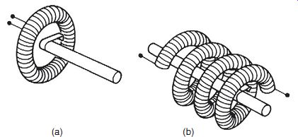
Figure 1
2.2 Rotational Differential Transformer
This is a special form of differential transformer that measures rotational rather than translational motion. The method of construction and connection of the windings is exactly the same as for the linear variable differential transformer, except that a specially shaped core is used that varies the mutual inductance between the windings as it rotates, as shown in Figure 2. Like its linear equivalent, the instrument suffers no wear in operation and therefore has a very long life with almost no maintenance requirements. It can also be modified for operation in harsh environments by enclosing the windings inside a protective enclosure. However, apart from the difficulty of avoiding some asymmetry between the secondary windings, great care has to be taken in these instruments to machine the core to exactly the right shape. In consequence, the inaccuracy cannot be reduced below +-1%, and even this level of accuracy is only obtained for limited excursions of the core _40_ away from the null position. For angular displacements of _60_ ,the typical inaccuracy rises to +-3%, and the instrument is unsuitable for measuring displacements greater than this.
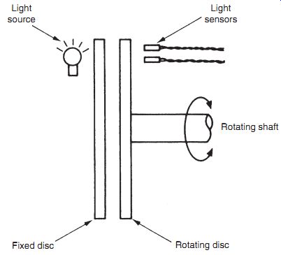
Figure 3
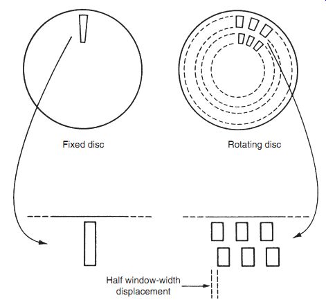
Figure 4
2.3 Incremental Shaft Encoders
Incremental shaft encoders are one of a class of encoder devices that give an output in digital form. They measure the instantaneous angular position of a shaft relative to some arbitrary datum point, but are unable to give any indication about the absolute position of a shaft. The principle of operation is to generate pulses as the shaft whose displacement is being measured rotates. These pulses are counted and total angular rotation is inferred from the pulse count. The pulses are generated either by optical or by magnetic means and are detected by suitable sensors. Of the two, the optical system is considerably less expensive and therefore much more common. Such instruments are very convenient for computer control applications, as the measurement is already in the required digital form and therefore the analogue-to-digital signal conversion process required for an analogue sensor is avoided.
An example of an optical incremental shaft encoder is shown in Figure 3. It can be seen that the instrument consists of a pair of discs, one of which is fixed and one of which rotates with the body whose angular displacement is being measured. Each disc is basically opaque but has a pattern of windows cut into it. The fixed disc has only one window and the light source is aligned with this so that the light shines through all the time. The second disc has two tracks of windows cut into it that are spaced equidistantly around the disc, as shown in Figure 4. Two light detectors are positioned beyond the second disc so that one is aligned with each track of windows. As the second disc rotates, light alternately enters and does not enter the detectors, as windows and then opaque regions of the disc pass in front of them. These pulses of light are fed to a counter, with the final count after motion has ceased corresponding to the angular position of the moving body relative to the starting position. The primary information about the magnitude of rotation is obtained by the detector aligned with the outer track of windows. However, the pulse count obtained from this gives no information about the direction of rotation. The necessary direction information is provided by the second, inner track of windows, which have an angular displacement with respect to the outer set of windows of half a window width. Pulses from the detector aligned with the inner track of windows therefore lag or lead the primary set of pulses according to the direction of rotation.
The maximum measurement resolution obtainable is limited by the number of windows that can be machined onto a disc. The maximum number of windows per track for a 150-mm diameter disc is 5000, which gives a basic angular measurement resolution of 1 in 5000. By using more sophisticated circuits that increment the count on both the rising and the falling edges of the pulses through the outer track of windows, it is possible to double the resolution to a maximum of 1 in 10,000. At the expense of even greater complexity in the counting circuit, it is also possible to include pulses from the inner track of windows in the count, so giving a maximum measurement resolution of 1 in 20,000.
Optical incremental shaft encoders are a popular instrument for measuring relative angular displacements and are very reliable. Problems of noise in the system giving false counts can sometimes cause difficulties, although this can usually be eliminated by squaring the output from the light detectors. Such instruments are found in many applications where rotational motion has to be measured. Incremental shaft encoders are also used commonly in circumstances where a translational displacement has been transformed to a rotational one by suitable gearing. One example of this practice is in measuring the translational motions in numerically controlled drilling machines. Typical gearing used for this would give one revolution per millimeter of translational displacement. By using an incremental shaft encoder with 1000 windows per track in such an arrangement, a measurement resolution of 1 mm is obtained.
2.4 Coded Disc Shaft Encoders
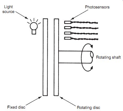
Figure 5

Figure 6
Unlike the incremental shaft encoder that gives a digital output in the form of pulses that have to be counted, the digital shaft encoder has an output in the form of a binary number of several digits that provides an absolute measurement of shaft position. Digital encoders provide high accuracy and reliability. They are particularly useful for computer control applications, but have a significantly higher cost than incremental encoders. Three different forms exist, using optical, electrical, and magnetic energy systems, respectively.
Optical digital shaft encoder
The optical digital shaft encoder is the least expensive form of encoder available and is the one used most commonly. It is found in a variety of applications; one where it is particularly popular is in measuring the position of rotational joints in robot manipulators. The instrument is similar in physical appearance to the incremental shaft encoder. It has a pair of discs (one movable and one fixed) with a light source on one side and light detectors on the other side, as shown in Figure 5. The fixed disc has a single window, and the principal way in which the device differs from the incremental shaft encoder is in the design of the windows on the movable disc, as shown in Figure 6. These are cut in four or more tracks instead of two and are arranged in sectors as well as tracks. An energy detector is aligned with each track, and these give an output of "1" when energy is detected and an output of "0" otherwise. The measurement resolution obtainable depends on the number of tracks used. For a four-track version, the resolution is 1 in 16, with progressively higher measurement resolution being attained as the number of tracks is increased. These binary outputs from the detectors are combined together to give a binary number of several digits. The number of digits corresponds to the number of tracks on the disc, which, in the example shown in Figure 6, is four. The pattern of windows in each sector is cut such that as that particular sector passes across the window in the fixed disc, the four energy detector outputs combine to give a unique binary number. In the binary-coded example shown in Figure 6, the binary number output increments by one as each sector in the rotating disc passes in turn across the window in the fixed disc. Thus the output from sector 1 is 0001, from sector 2 is 0010, from sector 3 is 0011, etc.
While this arrangement is perfectly adequate in theory, serious problems can arise in practice due to the manufacturing difficulty involved in machining the windows of the movable disc such that the edges of the windows in each track are aligned exactly with each other. Any misalignment means that, as the disc turns across the boundary between one sector and the next, the outputs from each track will switch at slightly different instants of time, and therefore the binary number output will be incorrect over small angular ranges corresponding to the sector boundaries. The worst error can occur at the boundary between sectors 7 and 8, where the output is switching from 0111 to 1000. If the energy sensor corresponding to the first digit switches before the others, then the output will be 1111 for a very small angular range of movement, indicating that sector 15 is aligned with the fixed disc rather than sector 7 or 8. This represents an error of 100% in the indicated angular position.
In practice, there are two ways that are used to overcome this difficulty. Both of these solutions involve an alteration to the manner in which windows are machined on the movable disc, as shown in Figure 7. The first method adds an extra outer track on the disc, known as an anti-ambiguity track, which consists of small windows that span a small angular range on either side of each sector boundary of the main track system. When energy sensors associated with this extra track sense energy, this is used to signify that the disc is aligned on a sector boundary and the output is unreliable. The second method is somewhat simpler and less expensive because it avoids the expense of machining the extra anti-ambiguity track. It does this by using a special code, known as the Gray code, to cut the tracks in each sector on the movable disk.
The Gray code is a special binary representation where only one binary digit changes in moving from one decimal number representation to the next, that is, from one sector to the next in the digital shaft encoder. The code is illustrated in Table 1.
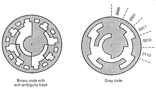
Figure 7
Table 1 The Gray Code
It is possible to manufacture optical digital shaft encoders with up to 21 tracks, which gives a measurement resolution of 1 part in 10^6 (about 1 second of arc). Unfortunately, a high cost is involved in the special photolithography techniques used to cut the windows in order to achieve such a measurement resolution, and very high-quality mounts and bearings are needed. Hence, such devices are very expensive.
Contacting (electrical) digital shaft encoder
The contacting digital shaft encoder consists of only one disc, which rotates with the body whose displacement is being measured. The disc has conducting and nonconducting segments instead of the transparent and opaque areas found on the movable disc of the optical form of instrument, but these are arranged in an identical pattern of sectors and tracks. The disc is charged to a low potential by an electrical brush in contact with one side of the disc, and a set of brushes on the other side of the disc measures the potential in each track. The output of each detector brush is interpreted as a binary value of "1" or "0" according to whether the track in that particular segment is conducting or not and hence whether a voltage is sensed or not. As for the case of the optical form of instrument, these outputs are combined together to give a multibit binary number. Contacting digital shaft encoders have a similar cost to the equivalent optical instruments and have operational advantages in severe environmental conditions of high temperature or mechanical shock.
They suffer from the usual problem of output ambiguity at the sector boundaries but this problem is overcome by the same methods used in optical instruments.
A serious problem in the application of contacting digital shaft encoders arises from their use of brushes. These introduce friction into the measurement system, and the combination of dirt and brush wear causes contact problems. Consequently, problems of intermittent output can occur, and such instruments generally have limited reliability and a high maintenance cost. Measurement resolution is also limited because of the lower limit on the minimum physical size of the contact brushes. The maximum number of tracks possible is 10, which limits the resolution to 1 part in 1000. Thus, contacting digital shaft encoders are normally only used where the environmental conditions are too severe for optical instruments.
Magnetic digital shaft encoder
Magnetic digital shaft encoders consist of a single rotatable disc, as in the contacting form of encoder discussed in the previous section. The pattern of sectors and tracks consists of magnetically conducting and nonconducting segments, and the sensors aligned with each track consist of small toroidal magnets. Each of these sensors has a coil wound on it that has a high or low voltage induced in it according to the magnetic field close to it.
This field is dependent on the magnetic conductivity of that segment of the disc closest to the toroid.
These instruments have no moving parts in contact and therefore have a similar reliability to optical devices. Their major advantage over optical equivalents is an ability to operate in very harsh environmental conditions. Unfortunately, the process of manufacturing and accurately aligning the toroidal magnet sensors required makes such instruments very expensive. Their use is therefore limited to a few applications where both high measurement resolution and also operation in harsh environments are required.
2.5 The Resolver
The resolver, also known as a synchro-resolver, is an electromechanical device that gives an analogue output by transformer action. Physically, resolvers resemble a small a.c. motor and have a diameter ranging from 10 to 100 mm. They are frictionless and reliable in operation because they have no contacting moving surfaces; consequently, they have a long life. The best devices give measurement resolutions of 0.1%.
Resolvers have two stator windings, which are mounted at right angles to one another, and a rotor, which can have either one or two windings. As the angular position of the rotor changes, the output voltage changes. The simpler configuration of a resolver with only one winding on a rotor is illustrated in Figure 8. This exists in two separate forms that are distinguished according to whether the output voltage changes in amplitude or changes in phase as the rotor rotates relative to the stator winding.
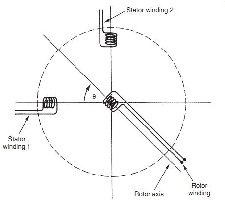
Figure 8
Varying amplitude output resolver
The stator of this type of resolver is excited with a single-phase sinusoidal voltage of frequency o, where the amplitudes in the two windings are given by:
V1 = V sin b () ; V2 = V cos b (), where V=Vs sin(ot).
The effect of this is to give a field at an angle of (b)p/2) relative to stator winding 1.
Suppose that the angle of the rotor winding relative to that of the stator winding is given by y.
Then the magnetic coupling between the windings is a maximum for y=(b)p/2) and a minimum for (y=b). The rotor output voltage is of fixed frequency and varying amplitude given by
Vo = KVs sin b _ y () sin ot ():
This relationship between shaft angle position and output voltage is nonlinear, but approximate linearity is obtained for small angular motions where |b_y|<15 _.
Intelligent versions of this type of resolver are available that use a microprocessor to process the sine and cosine outputs. This can improve the measurement resolution to 2 minutes of arc.
Varying phase output resolver
This is a less common form of resolver that is only used in a few applications. The stator windings are excited with a two-phase sinusoidal voltage of frequency o, and the instantaneous voltage amplitudes in the two windings are given by:
V1 = Vs sin ot () ; V2 = Vs sin ot ) p=2 ()= Vs cos ot ():
The net output voltage in the rotor winding is the sum of the voltages induced due to each stator winding. This is given by:
Vo = KVs sin ot () cos y () ) KVs cos ot () cos p=2 _ y ()
= KVs sin ot () cos y () ) cos ot () sin y () ½_
= KVs sin ot ) y ()
This represents a linear relationship between shaft angle and the phase shift of the rotor output relative to the stator excitation voltage. The accuracy of shaft rotation measurement depends on the accuracy with which the phase shift can be measured. This can be improved by increasing the excitation frequency, o, and it is possible to reduce inaccuracy down to _0.1%. However, increasing the excitation frequency also increases magnetizing losses. Consequently, a compromise excitation frequency of about 400 Hz is used.
2.6 The Synchro
Like the resolver, the synchro is a motor-like, electromechanical device with an analogue output. Apart from having three stator windings instead of two, the instrument is similar in appearance and operation to the resolver and has the same range of physical dimensions. The rotor usually has a dumbbell shape and, like the resolver, can have either one or two windings.
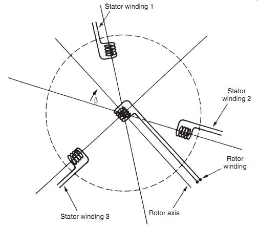
Figure 9
Synchros have been in use for many years for the measurement of angular positions, especially in military applications, and achieve similar levels of accuracy and measurement resolution to digital encoders. One common application is axis measurement in machine tools, where the translational motion of the tool is translated into a rotational displacement by suitable gearing. Synchros are tolerant to high temperatures, high humidity, shock, and vibration and are therefore suitable for operation in such harsh environmental conditions.
Some maintenance problems are associated with the slip ring and brush system used to supply power to the rotor. However, the only major source of error in the instrument is asymmetry in the windings, and a reduction of measurement inaccuracy down to +-0.5% is easily achievable.
Figure 9 shows the simpler form of a synchro with a single rotor winding. If an a.c. excitation voltage is applied to the rotor via slip rings and brushes, this sets up a certain pattern of fluxes and induced voltages in the stator windings by transformer action. For a rotor excitation voltage, Vr, given by Vr = V sin ot () the voltages induced in the three stator windings are:
V1 = V sin ot () sin b () ;V2 = V sin ot () sin b ) 2p=3 () ;
V3 = V sin ot () sin b _ 2p=3 ()
where b is the angle between the rotor and stator windings.
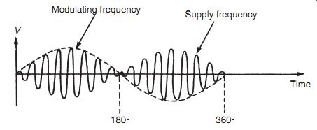
Figure 10
If the rotor is turned at constant velocity through one full revolution, the voltage waveform induced in each stator winding is as shown in Figure 10. This has the form of a carrier modulated waveform, in which the carrier frequency corresponds to the excitation frequency, o.
It follows that if the rotor is stopped at any particular angle, b', the peak-to-peak amplitude of the stator voltage is a function of b'. If therefore the stator winding voltage is measured, generally as its root-mean-squared (r.m.s.) value, this indicates the magnitude of the rotor rotation away from the null position. The direction of rotation is determined by the phase difference between the stator voltages, which is indicated by their relative instantaneous magnitudes.
Although a single synchro is able to measure an angular displacement by itself, it is much more common to find a pair of them used for this purpose. When used in pairs, one member of the pair is known as the synchro transmitter and the other as the synchro transformer, and the two sets of stator windings are connected together, as shown in Figure 11. Each synchro is of the form shown in Figure 9, but the rotor of the transformer is fixed for displacement-measuring applications. A sinusoidal excitation voltage is applied to the rotor of the transmitter, setting up a pattern of fluxes and induced voltages in the transmitter stator windings. These voltages are transmitted to the transformer stator windings, where a similar flux pattern is established. This in turn causes a sinusoidal voltage to be induced in the fixed transformer rotor winding. For an excitation voltage, V sin(ot), applied to the transmitter rotor, the voltage measured in the transformer rotor is given by Vo = V sin ot () sin y ();
...where y is the relative angle between the two rotor windings.
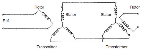
Figure 11
Apart from their use as a displacement transducer, such synchro pairs are commonly used to transmit angular displacement information over some distance, for instance, to transmit gyro compass measurements in an aircraft to remote meters. They are also used for load positioning, allowing a load connected to the transformer rotor shaft to be controlled remotely by turning the transmitter rotor. For these applications, the transformer rotor is free to rotate, and it is also damped to prevent oscillatory motions. In the simplest arrangement, a common sinusoidal excitation voltage is applied to both rotors. If the transmitter rotor is turned, this causes an imbalance in the magnetic flux patterns and results in a torque on the transformer rotor that tends to bring it into line with the transmitter rotor. This torque is typically small for small displacements, so this technique is only useful if the load torque on the transformer shaft is very small. In other circumstances, it is necessary to incorporate the synchro pair within a servomechanism, where the output voltage induced in the transformer rotor winding is amplified and applied to a servomotor that drives the transformer rotor shaft until it is aligned with the transmitter shaft.
2.7 The Induction Potentiometer
The induction potentiometer belongs to the same class of instruments as resolvers and synchros.
It only has one rotor winding and one stator winding, but otherwise it is of similar size and appearance to other devices in this class of electromechanical, angular position measuring instruments. A single-phase sinusoidal excitation is applied to the rotor winding, which causes an output voltage in the stator winding through the mutual inductance linking the two windings.
The magnitude of this induced stator voltage varies with rotation of the rotor. The variation of the output with rotation is naturally sinusoidal if the coils are wound such that their field is concentrated at one point, and only small excursions can be made away from the null position if the output relationship is to remain approximately linear. However, if the rotor and stator windings are distributed around the circumference in a special way, an approximately linear relationship for angular displacements of up to +90 Can be obtained.
2.8 The Rotary Inductosyn
This instrument is similar in operation to the linear inductosyn, except that it measures rotary displacements and has tracks that are arranged radially on two circular discs, as shown in Figure 12. Typical diameters of the instrument vary between 75 and 300 mm. The larger versions give a measurement resolution of up to 0.05 second of arc. However, like its linear equivalent, the rotary inductosyn has a very small measurement range. Therefore, a lower resolution, rotary displacement transducer with a larger measurement range must be used in conjunction with it.

Figure 12
2.9 Gyroscopes
Gyroscopes measure both absolute angular displacement and absolute angular velocity.
Until recently, the mechanical, spinning-wheel gyroscope had a dominant position in the marketplace. However, this position is now being challenged by optical gyroscopes.
Mechanical gyroscopes
Mechanical gyroscopes consist essentially of a large, motor-driven wheel whose angular momentum is such that the axis of rotation tends to remain fixed in space, thus acting as a reference point. The gyro frame is attached to the body whose motion is to be measured. The output is measured in terms of the angle between the frame and the axis of the spinning wheel.
Two different forms of mechanical gyroscopes are used for measuring angular displacement- the free gyro and the rate-integrating gyro. A third type of mechanical gyroscope, the rate gyro, measures angular velocity and is described in Sub-Section 3.
The free gyroscope is illustrated in Figure 13. This measures the absolute angular rotation about two perpendicular axes of the body to which its frame is attached. Two alternative methods of driving the wheel are used in different versions of the instrument. One of these is to enclose the wheel in stator-like coils that are excited with a sinusoidal voltage. A voltage is applied to the wheel via slip rings at both ends of the spindle carrying the wheel. The wheel behaves as a rotor, and motion is produced by motor action. The other, less common, method is to fix vanes on the wheel, which is then driven by directing a jet of air onto the vanes.
The free gyroscope can measure angular displacements of up to 10_ with a high accuracy. For greater angular displacements, interaction between the measurements on the two perpendicular axes starts to cause a serious loss of accuracy. The physical size of the coils in the motor-action driven system also limits the measurement range to 10_. For these reasons, this type of gyroscope is only suitable for measuring rotational displacements of up to 10_ . A further operational problem of free gyroscopes is the presence of angular drift (precession) due to bearing friction torque. This has a typical magnitude of 0.5_ per minute and means that the instrument can only be used over short time intervals of say 5 minutes. This time duration can be extended if the angular momentum of the spinning wheel is increased.
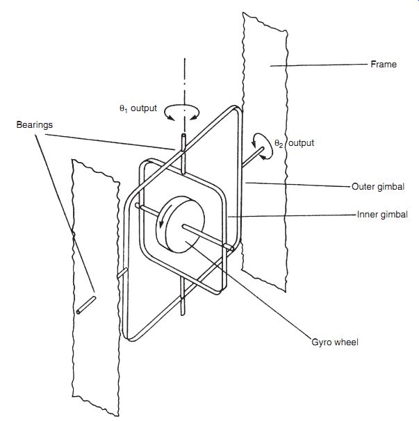
Figure 13
A major application of the free gyroscope is in inertial navigation systems. Only two free gyros mounted along orthogonal axes are needed to monitor motions in three dimensions because each instrument measures displacement about two axes. The limited angular range of measurement is not usually a problem in such applications, as control action prevents the error in the direction of motion about any axis ever exceeding one or two degrees. However, precession is a much greater problem, and, for this reason, the rate-integrating gyro is used much more commonly.
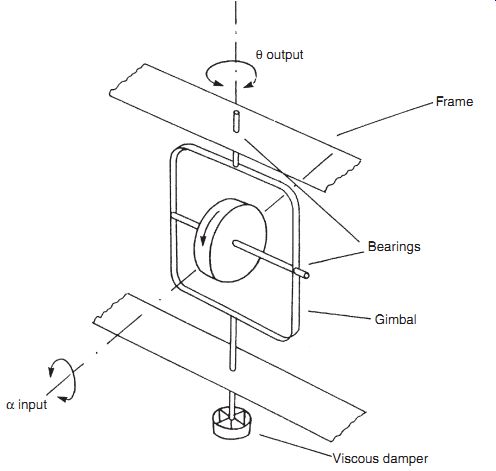
Figure 14
The rate-integrating gyroscope, or integrating gyro as it is commonly known, is illustrated in Figure 14. It measures angular displacements about a single axis only, and therefore three instruments are required in a typical inertial navigation system. The major advantage of the instrument over the free gyro is the almost total absence of precession, with typical specifications quoting drifts of only 0.01_/hour. The instrument has a first-order type of response given by yo yi D ()= K tD ) 1
(eqn. 1)
...where K=H/b, t=M/b, yi is the input angle, yo is the output angle, D is the D operator, H is the angular momentum, M is the moment of inertia of the system about the measurement axis, and b is the damping coefficient.
Inspection of Equation (1) shows that to obtain a high value of measurement sensitivity, K,a high value of H and a low value of b are required. A large H is normally obtained by driving the wheel with a hysteresis-type motor revolving at high speeds of up to 24,000 rpm. However, damping coefficient b can only be reduced so far because a small value of b results in a large value for the system time constant, t, and an unacceptably low speed of system response.
Therefore, the value of b has to be chosen as a compromise between these constraints.
In addition to their use as a fixed reference in inertial guidance systems, integrating gyros are also used commonly within aircraft autopilot systems and in military applications such as stabilizing weapon systems in tanks.
Optical gyroscopes
Optical gyroscopes are a relatively recent development and come in two forms-ring laser gyroscope and fiber-optic gyroscope.
The ring laser gyroscope consists of a glass ceramic chamber containing a helium-neon gas mixture in which two laser beams are generated by a single anode/twin cathode system, as shown in Figure 15. Three mirrors, supported by the ceramic block and mounted in a triangular arrangement, direct the pair of laser beams around the cavity in opposite directions.
Any rotation of the ring affects the coherence of the two beams, raising the frequency of one and lowering the frequency of the other. The clockwise and anticlockwise beams are directed into a photodetector that measures the beat frequency according to the frequency difference, which is proportional to the angle of rotation. The advantages of the ring laser gyroscope over traditional, mechanical gyroscopes are considerable. The measurement accuracy obtained is substantially better than that afforded by mechanical gyros in a similar price range. The device is also considerably smaller physically, which is of considerable benefit in many applications.
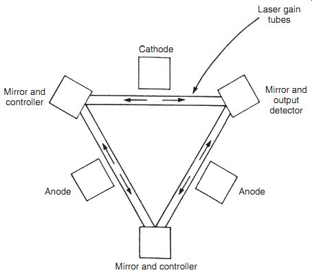
Figure 15
The fiber-optic gyroscope measures angular velocity and is described in Sub-Section 3.
2.10 Choice between Rotational Displacement Transducers
Choice between the various rotational displacement transducers that might be used in any particular measurement situation depends first of all on whether absolute measurement of angular position is required or whether the measurement of rotation relative to some arbitrary starting point is acceptable. Other factors affecting the choice between instruments are the required measurement range, resolution of the transducer, and measurement accuracy afforded.
Where only measurement of relative angular position is required, the incremental encoder is a very suitable instrument. The best commercial instruments of this type can measure rotations to a resolution of 1 part in 20,000 of a full revolution, and the measurement range is an infinite number of revolutions. Instruments with such a high measurement resolution are very expensive, but much less expensive versions are available according to what lower level of measurement resolution is acceptable.
All the other instruments presented in this SECTION provide an absolute measurement of angular position. The required measurement range is a dominant factor in the choice between these. If this exceeds one full revolution, then the only instrument available is the helical potentiometer. Such devices can measure rotations of up to 60 full turns, but are expensive because the procedure involved in manufacturing a helical resistance element to a reasonable standard of accuracy is difficult.
For measurements of less than one full revolution, the range of available instruments widens.
The least expensive one available is the circular potentiometer, but much better measurement accuracy and resolution are obtained from coded-disc encoders. The least expensive of these is the optical form, but certain operating environments necessitate the use of the alternative contacting (electrical) and magnetic versions. All types of coded disc encoders are very reliable and are particularly attractive in computer control schemes, as the output is in digital form. A varying phase output resolver is yet another instrument that can measure angular displacements up to one full revolution in magnitude. Unfortunately, this instrument is expensive because of the complicated electronics incorporated to measure the phase variation and convert it to a varying amplitude output signal, and hence it is no longer in common use.
An even greater range of instruments becomes available as the required measurement range is reduced further. These include the synchro (_90_ ), the varying amplitude output resolver (_90_ ), the induction potentiometer (_90_ ), and the differential transformer (_40_ ). All these instruments have a high reliability and a long service life.
Finally, two further instruments are available for satisfying special measurement requirements-the rotary inductosyn and the gyroscope. The rotary inductosyn is used in applications where very high measurement resolution is required, although the measurement range afforded is extremely small and a coarser resolution instrument must be used in parallel with it to extend the measurement range. Gyroscopes, in both mechanical and optical forms, are used to measure small angular displacements up to _10_ in magnitude in inertial navigation systems and similar applications.
2.11 Calibration of Rotational Displacement Transducers
The coded disc shaft encoder is normally used for the calibration of rotary potentiometers and differential transformers. A typical model provides a reference standard with a measurement uncertainty of +-0.1% of the full-scale reading. If greater accuracy is required, for example, in calibrating encoders of lesser accuracy, encoders with measurement uncertainty down to +-0.0001% of the full-scale reading can be obtained and used as a reference standard, although these have a very high associated cost.
3. Rotational Velocity
The main application of rotational velocity transducers is in speed control systems. They also provide the usual means of measuring translational velocities, which are transformed into rotational motions for measurement purposes by suitable gearing. Many different instruments and techniques are available for measuring rotational velocity as presented here.
3.1 Digital Tachometers
Digital tachometers or, to give them their proper title, digital tachometric generators are usually noncontact instruments that sense the passage of equally spaced marks on the surface of a rotating disk or shaft. Measurement resolution is governed by the number of marks around the circumference. Various types of sensors are used, such as optical, inductive, and magnetic ones.
As each mark is sensed, a pulse is generated and input to an electronic pulse counter. Usually, velocity is calculated in terms of the pulse count in unit time, which of course only yields information about the mean velocity. If the velocity is changing, instantaneous velocity can be calculated at each instant of time that an output pulse occurs, using the scheme shown in Figure 16. In this circuit, each pulse from the transducer initiates the transfer of a train of clock pulses from a 1-MHz clock into a counter. Control logic resets the counter and updates the digital output value after receipt of each transducer pulse. The measurement resolution of this system is highest when the speed of rotation is low.
Optical sensing
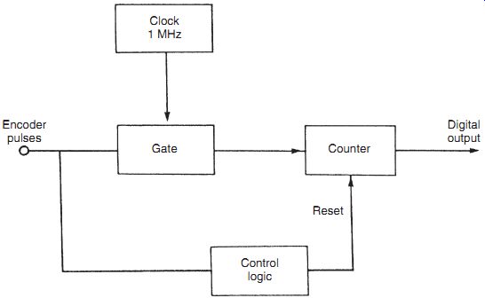
Figure 16
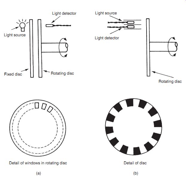
Figure 17
Digital tachometers with optical sensors are often known as optical tachometers. Optical pulses can be generated by one of the two alternative photoelectric techniques illustrated in Figure 17. In the scheme shown in Figure 17a, pulses are produced as windows in a slotted disc pass in sequence between a light source and a detector. The alternative scheme, shown in Figure 17b, has both a light source and a detector mounted on the same side of a reflective disc that has black sectors painted onto it at regular angular intervals. Light sources are normally either lasers or light-emitting diodes, with photodiodes and phototransistors being used as detectors. Optical tachometers yield better accuracy than other forms of digital tachometers. However, they are less reliable than other forms because dust and dirt can block light paths.
Inductive sensing
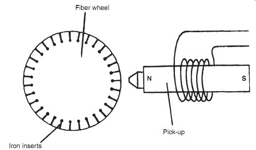
Figure 18
Variable reluctance velocity transducers, also known as induction tachometers, area form of digital tachometer that use inductive sensing. They are widely used in the automotive industry within antiskid devices, antilock braking systems, and traction control. One relatively simple and inexpensive form of this type of device was described earlier in Section 4 (Figure 2). A more sophisticated version, shown in Figure 18, has a rotating disc constructed from a bonded fiber material into which soft iron poles are inserted at regular intervals around its periphery. The sensor consists of a permanent magnet with a shaped pole piece, which carries a wound coil. The distance between the pickup and the outer perimeter of the disc is typically 0.5 mm. As the disc rotates, the soft iron inserts on the disc move in turn past the pickup unit. As each iron insert moves toward the pole piece, the reluctance of the magnetic circuit increases and hence the flux in the pole piece also increases. Similarly, the flux in the pole piece decreases as each iron insert moves away from the sensor. The changing magnetic flux inside the pickup coil causes a voltage to be induced in the coil whose magnitude is proportional to the rate of change of flux. This voltage is positive while the flux is increasing and negative while it is decreasing. Thus, the output is a sequence of positive and negative pulses whose frequency is proportional to the rotational velocity of the disc. The maximum angular velocity that the instrument can measure is limited to about 10,000 r.p.m. because of the finite width of the induced pulses. As the velocity increases, the distance between pulses is reduced; at a certain velocity, the pulses start to overlap. At this point, the pulse counter ceases to be able to distinguish separate pulses. The optical tachometer has significant advantages in this respect, as the pulse width is much narrower, allowing measurement of higher velocities.
A simpler and less expensive form of variable reluctance transducer also exists that uses a ferromagnetic gear wheel in place of a fiber disc. The motion of the tip of each gear tooth toward and away from the pickup unit causes a similar variation in the flux pattern to that produced by iron inserts in the fiber disc. However, pulses produced by these means are less sharp and, consequently, the maximum angular velocity measurable is lower.
Magnetic (Hall-effect) sensing
The rotating element in Hall-effect or magnetostrictive tachometers has a very simple design in the form of a toothed metal gear wheel. The sensor is a solid-state, Hall-effect device that is placed between the gear wheel and a permanent magnet. When an inter-tooth gap on the gear wheel is adjacent to the sensor, the full magnetic field from the magnet passes through it.
Later, as a tooth approaches the sensor, the tooth diverts some of the magnetic field, and so the field through the sensor is reduced. This causes the sensor to produce an output voltage proportional to the rotational speed of the gear wheel.
3.2 Stroboscopic Methods
The stroboscopic technique of rotational velocity measurement operates on a similar physical principle to digital tachometers except that the pulses involved consist of flashes of light generated electronically and whose frequency is adjustable so that it can be matched with the frequency of occurrence of some feature on the rotating body being measured. This feature can either be some naturally occurring one, such as gear teeth or spokes of a wheel, or be an artificially created pattern of black and white stripes. In either case, the rotating body appears stationary when frequencies of the light pulses and body features are in synchronism. Flashing rates available in commercial stroboscopes vary from 110 up to 150,000 per minute according to the range of velocity measurement required, and typical measurement inaccuracy is +-1% of the reading. The instrument is usually in the form of a hand-held device that is pointed toward the rotating body.
It must be noted that measurement of the flashing rate at which the rotating body appears stationary does not automatically indicate the rotational velocity, because synchronism also occurs when the flashing rate is some integral sub-multiple of the rotational speed. The practical procedure followed is therefore to adjust the flashing rate until synchronism is obtained at the largest flashing rate possible, R1. The flashing rate is then decreased carefully until synchronism is again achieved at the next lower flashing rate, R2. The rotational velocity is then given by
V = R1R2 R1 _ R2:
3.3 Analogue Tachometers
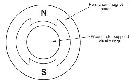
Figure 19
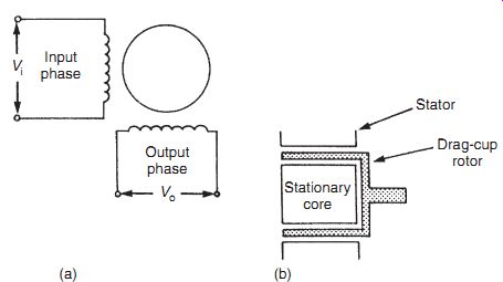
Figure 20
Analogue tachometers are less accurate than digital tachometers but are nevertheless still used successfully in many applications. Various forms exist.
The d.c. tachometer has an output approximately proportional to its speed of rotation. Its basic structure is identical to that found in a standard d.c. generator used for producing power and is shown in Figure 19. Both permanent magnet types and separately excited field types are used. However, certain aspects of the design are optimized to improve its accuracy as a speed-measuring instrument. One significant design modification is to reduce the weight of the rotor by constructing the windings on a hollow fiberglass shell. The effect of this is to minimize any loading effect of the instrument on the system being measured. The d.c. output voltage from the instrument is of a relatively high magnitude, giving a high measurement sensitivity that is typically 5 volts per 1000 r.p.m. The direction of rotation is determined by the polarity of the output voltage. A common range of measurement is 0-6000 r.p.m. Maximum nonlinearity is usually about +-1% of the full-scale reading. One problem with these devices that can cause difficulties under some circumstances is the presence of an a.c. ripple in the output signal. The magnitude of this can be up to 2% of the output d.c. level.
The a.c. tachometer has an output approximately proportional to rotational speed like the d.c. tachogenerator. Its mechanical structure takes the form of a two-phase induction motor, with two stator windings and (usually) a drag-cup rotor, as shown in Figure 20. One of the stator windings is excited with an a.c. voltage, and the measurement signal is taken from the output voltage induced in the second winding. The magnitude of this output voltage is zero when the rotor is stationary, and otherwise is proportional to the angular velocity of the rotor.
The direction of rotation is determined by the phase of the output voltage, which switches by 180 deg. as the direction reverses. Therefore, both the phase and the magnitude of the output voltage have to be measured. A typical range of measurement is 0-4000 r.p.m., with an inaccuracy of +-0.05% of full-scale reading. Less expensive versions with a squirrel cage rotor also exist, but measurement inaccuracy in these is typically +-0.25%.
The drag-cup tachometer, also known as an eddy-current tachometer, has a central spindle carrying a permanent magnet that rotates inside a nonmagnetic drag cup consisting of a cylindrical sleeve of electrically conductive material, as shown in Figure 21. As the spindle and magnet rotate, voltage is induced that causes circulating eddy currents in the cup. These currents interact with the magnetic field from the permanent magnet and produce a torque. In response, the drag cup turns until the induced torque is balanced by the torque due to the restraining springs connected to the cup. When equilibrium is reached, angular displacement of the cup is proportional to the rotational velocity of the central spindle. The instrument has a typical measurement inaccuracy of _0.5% and is used commonly in the speedometers of motor vehicles and also as a speed indicator for aero-engines. It is capable of measuring velocities up to 15,000 r.p.m.
Analogue output forms of the variable reluctance velocity transducer (see Sub-Section 3.1) also exist in which output voltage pulses are converted into an analogue, varying-amplitude, d.c. voltage by means of a frequency-to-voltage converter circuit. However, the measurement accuracy is inferior to digital output forms.
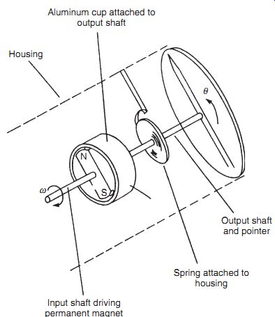
Figure 21
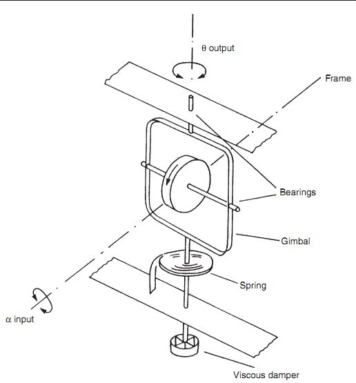
Figure 22
3.4 The Rate Gyroscope
The rate gyro, illustrated in Figure 22, has an almost identical construction to the rate integrating gyro (Figure 14) and differs only by including a spring system that acts as an additional restraint on the rotational motion of the frame. The instrument measures the absolute angular velocity of a body and is widely used for generating stabilizing signals within vehicle navigation systems. The typical measurement resolution given by the instrument is 0.01_/s, and rotation rates up to 50_/s can be measured. The angular velocity, a, of the body is related to the angular deflection of the gyroscope, y, by the equation:
y a D ()= H MD2 ) bD ) K , (eqn. 2)
where H is the angular momentum of the spinning wheel, M is the moment of inertia of the system, b is the viscous damping coefficient, K is the spring constant, and D is the D operator.
This relationship [Equation (2)] is a second-order differential equation, and we must consequently expect the device to have a response typical of second-order instruments, as discussed in SECTION 2. Therefore, the instrument must be designed carefully so that the output response is neither oscillatory nor too slow in reaching a final reading. To assist in the design process, it is useful to re-express Equation (2) in the following form:
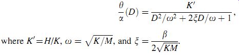
(eqn. 3)
The static sensitivity of the instrument, K0 , is made as large as possible by using a high-speed motor to spin the wheel and so make H high. Reducing the spring constant K further improves the sensitivity, but this cannot be reduced too far as it makes the resonant frequency o of the instrument too small. The value of b is usually chosen such that the damping ratio x is as close to 0.7 as possible.
3.5 Fiber-Optic Gyroscope
This is a relatively new instrument that makes use of fiber-optic technology. Incident light from a source is separated by a beam splitter into a pair of beams, a and b, as shown in Figure 23. These travel in opposite directions around an fiber-optic coil (which may be several hundred meters long) and emerge from the coil as beams marked a' and b'. The beams a' and b' are directed by the beam splitter into an interferometer. Any motion of the coil causes a phase shift between a' and b', which is detected by the interferometer.
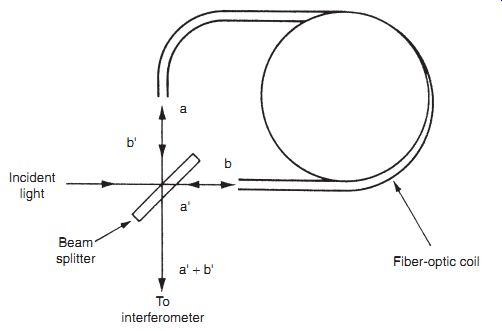
Figure 23
3.6 Differentiation of Angular Displacement Measurements
Angular velocity measurements can be obtained by differentiating the output signal from angular displacement transducers. Unfortunately, the process of differentiation amplifies any noise in the measurement signal, and therefore this technique has been used only rarely in the past. However, the technique has become more feasible with the advent of intelligent instruments. For example, using an intelligent instrument to differentiate and process the output from a resolver can produce a velocity measurement with a maximum inaccuracy of +-1%.
3.7 Integration of Output from an Accelerometer
In measurement systems that already contain an angular acceleration transducer, it is possible to obtain a velocity measurement by integrating the acceleration measurement signal.
This produces a signal of acceptable quality, as the process of integration attenuates any measurement noise. However, the method is of limited value in many measurement situations because the measurement obtained is the average velocity over a period of time rather than a profile of the instantaneous velocities as motion takes place along a particular path.
3.8 Choice between Rotational Velocity Transducers
Choice between different rotational velocity transducers is influenced strongly by whether an analogue or digital form of output is required. Digital output instruments are now widely used and a choice has to be made among the variable reluctance transducer, devices using electronic light pulse-counting methods, and the stroboscope. The first two of these are used to measure angular speeds up to about 10,000 r.p.m. and the last one can measure speeds up to 25,000 r.p.m.
Probably the most common form of analogue output device used is the d.c. tachometer. This is a relatively simple device that measures speeds up to about 5000 r.p.m. with a maximum inaccuracy of +-1%. Where better accuracy is required within a similar range of speed measurement, a.c. tachometers are used. The squirrel cage rotor type has an inaccuracy of only +-0.25%, and drag-cup rotor types can have inaccuracies as low as +-0.05%.
The drag-cup tachometer also has an analogue output, but has a typical inaccuracy of +-5%.
However, it is inexpensive and therefore suitable for use in vehicle speedometers where an inaccuracy of +-5% is normally acceptable.
3.9 Calibration of Rotational Velocity Transducers
The main device used as a calibration standard for rotational velocity transducers is a stroboscope. Provided the flash frequency of the reference stroboscope is calibrated properly, it is possible to provide velocity measurements where the inaccuracy is less than +-0.1%.
4. Rotational Acceleration
Rotational accelerometers work on very similar principles to translational motion accelerometers. They consist of a rotatable mass mounted inside a housing attached to the accelerating, rotating body. Rotation of the mass is opposed by a torsional spring and damping. Any acceleration of the housing causes a torque, J€ y, on the mass. This torque is opposed by a backward torque due to the torsional spring and in equilibrium:
J€ y = Ky and hence: € y = ky=J:
A damper is usually included in the system to avoid undying oscillations in the instrument.
This adds an additional backward torque, B_ y, to the system and the equation of motion becomes J€ y = B_ y ) Ky:
Different manufacturers produce accelerometers that measure the angular displacement of the mass within the accelerometer in different ways. However, it should be noted that the number of manufacturers producing rotational accelerometers is substantially less than the number manufacturing translational motion accelerometers because the requirement to measure rotational acceleration occurs much less frequently than requirements to measure translational acceleration.
4.1 Calibration of Rotational Accelerometers
This is normally carried out by comparison with a reference standard rotational accelerometer.
The task is usually delegated to specialist calibration companies or accelerometer manufacturers because of the relatively small number of applications for rotational accelerometers and the corresponding shortage of personnel having the necessary calibration skills.
5. Summary
Having discussed sensors for measuring translational motion in the previous SECTION, this SECTION has been concerned with the measurement of the three aspects-displacement, velocity, and acceleration-of rotational motion. Starting with sensors for measuring rotation displacement, we first discussed circular and helical potentiometers. Next we considered the merits of the rotational differential transformer, incremental shaft encoder, coded disc shaft encoder, resolver, synchro, induction potentiometer, rotary inductosyn, and both free and rate-integrating gyroscopes.
Moving on to the measurement of rotational velocity, we first explored the various forms of digital tachometers available. Discussion then moved on to stroboscopic methods, followed by a review of analogue tachometers, which we noted were less accurate than digital tachometers but still in fairly widespread use. Next, we covered the two forms of gyroscopes that measure rotational velocity-rate gyro and fiber-optic gyro. Finally, we found that a velocity measurement could be obtained by differentiating an angular displacement measurement or by integrating an acceleration measurement. However, we noted that while the latter is acceptable because the process of integration attenuates any measurement noise, the differentiation technique is not used unless done within an intelligent instrument that can deal with the noise amplification that is inherent when measurements are obtained via differentiation.
Our final subject in the SECTION was the measurement of rotational acceleration. We noted that rotational accelerometers worked on very similar principles to their translational motion counterparts, while observing that the requirement of measure rotational acceleration did not commonly arise.
6. Problems
1. Using simple sketches to support your explanation, explain the mode of operation and characteristics of the following devices: circular potentiometer, helical potentiometer, and rotary differential transformer.
2. Sketch an incremental shaft encoder. Explain what it measures and how it works. What special design features can be implemented to increase the measurement resolution of a disc of a given diameter?
3. What is a coded disc shaft encoder? How does its output differ from that of an incremental shaft encoder? What are the main types of coded disc shaft encoders?
4. Discuss the mode of operation of an optical coded disc shaft encoder, illustrating your discussion by means of a sketch.
5. What is the main consequence of any misalignment of the windows in an optical coded disc shaft encoder? Describe two ways in which the problem caused by window misalignment can be overcome.
6. Explain what a resolver is in the context of rotational position measurement. Discuss the two alternative forms of resolvers that exist.
7. How does a synchro work? Illustrate your explanation with a simple sketch.
8. What is a gyroscope? Discuss the characteristics and mode of operation of three kinds of gyroscopes that can measure angular position.
9. Explain the mode of construction and characteristics of each of the following: digital tachometer, optical tachometer, induction tachometer, and Hall-effect tachometer.
10. Discuss the characteristics of stroboscopic methods of measuring rotational velocity.
11. What are the main types of analogue tachometers available? Discuss the main characteristics of each.
12. How does a rate gyroscope work? What is its main application?
PREV. | NEXT