AMAZON multi-meters discounts AMAZON oscilloscope discounts
1. Introduction
We have already been introduced to the subject of measurement uncertainty in the last SECTION, in the context of defining the accuracy characteristic of a measuring instrument. The existence of measurement uncertainty means that we would be entirely wrong to assume (although the uninitiated might assume this) that the output of a measuring instrument or larger measurement system gives the exact value of the measured quantity. Measurement errors are impossible to avoid, although we can minimize their magnitude by good measurement system design accompanied by appropriate analysis and processing of measurement data.
We can divide errors in measurement systems into those that arise during the measurement process and those that arise due to later corruption of the measurement signal by induced noise during transfer of the signal from the point of measurement to some other point. This SECTION considers only the first of these, with discussion on induced noise being deferred to SECTION 6.
It is extremely important in any measurement system to reduce errors to the minimum possible level and then to quantify the maximum remaining error that may exist in any instrument output reading. However, in many cases, there is a further complication that the final output from a measurement system is calculated by combining together two or more measurements of separate physical variables. In this case, special consideration must also be given to determining how the calculated error levels in each separate measurement should be combined to give the best estimate of the most likely error magnitude in the calculated output quantity. This subject is considered in Section 7.
The starting point in the quest to reduce the incidence of errors arising during the measurement process is to carry out a detailed analysis of all error sources in the system. Each of these error sources can then be considered in turn, looking for ways of eliminating or at least reducing the magnitude of errors. Errors arising during the measurement process can be divided into two groups, known as systematic errors and random errors.
Systematic errors describe errors in the output readings of a measurement system that are consistently on one side of the correct reading, that is, either all errors are positive or are all negative. (Some books use alternative name bias errors for systematic errors, although this is not entirely incorrect, as systematic errors include errors such as sensitivity drift that are not biases.) Two major sources of systematic errors are system disturbance during measurement and the effect of environmental changes (sometimes known as modifying inputs), as discussed in Sections 4.1 and 4.2. Other sources of systematic error include bent meter needles, use of uncalibrated instruments, drift in instrument characteristics, and poor cabling practices.
Even when systematic errors due to these factors have been reduced or eliminated, some errors remain that are inherent in the manufacture of an instrument. These are quantified by the accuracy value quoted in the published specifications contained in the instrument data sheet.
Random errors, which are also called precision errors in some books, are perturbations of the measurement either side of the true value caused by random and unpredictable effects, such that positive errors and negative errors occur in approximately equal numbers for a series of measurements made of the same quantity. Such perturbations are mainly small, but large perturbations occur from time to time, again unpredictably. Random errors often arise when measurements are taken by human observation of an analogue meter, especially where this involves interpolation between scale points. Electrical noise can also be a source of random errors. To a large extent, random errors can be overcome by taking the same measurement a number of times and extracting a value by averaging or other statistical techniques, as discussed in Section 5. However, any quantification of the measurement value and statement of error bounds remains a statistical quantity. Because of the nature of random errors and the fact that large perturbations in the measured quantity occur from time to time, the best that we can do is to express measurements in probabilistic terms: we may be able to assign a 95 or even 99% confidence level that the measurement is a certain value within error bounds of, say, +-1%, but we can never attach a 100% probability to measurement values that are subject to random errors. In other words, even if we say that the maximum error is +-0.5 of the measurement reading, there is still a 1% chance that the error is greater than +-0.5.
Finally, a word must be said about the distinction between systematic and random errors. Error sources in the measurement system must be examined carefully to determine what type of error is present, systematic or random, and to apply the appropriate treatment. In the case of manual data measurements, a human observer may make a different observation at each attempt, but it is often reasonable to assume that the errors are random and that the mean of these readings is likely to be close to the correct value. However, this is only true as long as the human observer is not introducing a parallax-induced systematic error as well by persistently reading the position of a needle against the scale of an analog meter from one side rather than from directly above. A human-induced systematic error is also introduced if an instrument with a first-order characteristic is read before it has settled to its final reading.
Wherever a systematic error exists alongside random errors, correction has to be made for the systematic error in the measurements before statistical techniques are applied to reduce the effect of random errors.
2. Sources of Systematic Error
The main sources of systematic error in the output of measuring instruments can be summarized as
• effect of environmental disturbances, often called modifying inputs
• disturbance of the measured system by the act of measurement
• changes in characteristics due to wear in instrument components over a period of time
• resistance of connecting leads
These various sources of systematic error, and ways in which the magnitude of the errors can be reduced, are discussed here.
2.1 System Disturbance due to Measurement
Disturbance of the measured system by the act of measurement is a common source of systematic error. If we were to start with a beaker of hot water and wished to measure its temperature with a mercury-in-glass thermometer, then we would take the thermometer, which would initially be at room temperature, and plunge it into the water. In so doing, we would be introducing a relatively cold mass (the thermometer) into the hot water and a heat transfer would take place between the water and the thermometer. This heat transfer would lower the temperature of the water. While the reduction in temperature in this case would be so small as to be undetectable by the limited measurement resolution of such a thermometer, the effect is finite and clearly establishes the principle that, in nearly all measurement situations, the process of measurement disturbs the system and alters the values of the physical quantities being measured.
A particularly important example of this occurs with the orifice plate. This is placed into a fluid-carrying pipe to measure the flow rate, which is a function of the pressure that is measured either side of the orifice plate. This measurement procedure causes a permanent pressure loss in the flowing fluid. The disturbance of the measured system can often be very significant.
Thus, as a general rule, the process of measurement always disturbs the system being measured.
The magnitude of the disturbance varies from one measurement system to the next and is affected particularly by the type of instrument used for measurement. Ways of minimizing disturbance of measured systems are important considerations in instrument design. However, an accurate understanding of the mechanisms of system disturbance is a prerequisite for this.
Measurements in electric circuits
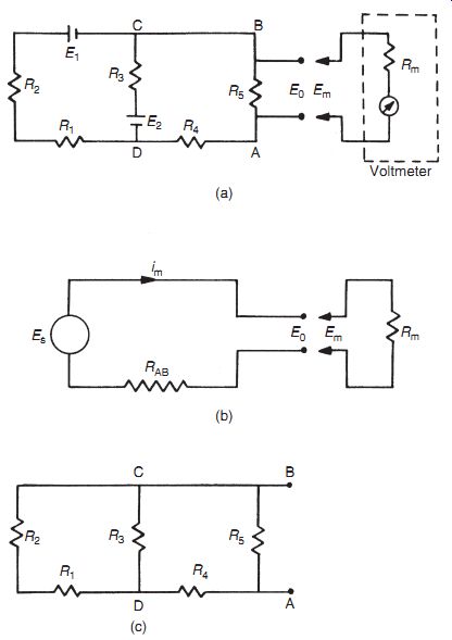
Figure 1
In analyzing system disturbance during measurements in electric circuits, Thevenin's theorem (see Appendix 2) is often of great assistance. For instance, consider the circuit shown in Figure 1a in which the voltage across resistor R5 is to be measured by a voltmeter with resistance Rm. Here, Rm acts as a shunt resistance across R5, decreasing the resistance between points AB and so disturbing the circuit. Therefore, the voltage Em measured by the meter is not the value of the voltage Eo that existed prior to measurement. The extent of the disturbance can be assessed by calculating the open-circuit voltage Eo and comparing it with Em.
The ´venin's theorem allows the circuit of Figure 1a comprising two voltage sources and five resistors to be replaced by an equivalent circuit containing a single resistance and one voltage source, as shown in Figure 1b. For the purpose of defining the equivalent single resistance of a circuit by The ´venin's theorem, all voltage sources are represented just by their internal resistance, which can be approximated to zero, as shown in Figure 1c. Analysis proceeds by calculating the equivalent resistances of sections of the circuit and building these up until the required equivalent resistance of the whole of the circuit is obtained. Starting at C and D, the circuit to the left of C and D consists of a series pair of resistances (R1 and R2) in parallel with R1, and the equivalent resistance can be written as:
Moving now to A and B, the circuit to the left consists of a pair of series resistances (RCD and R4) in parallel with R5. The equivalent circuit resistance RAB can thus be written as:
Substituting for RCD using the expression derived previously, we obtain:

(eqn. 1)
Defining I as the current flowing in the circuit when the measuring instrument is connected to it, we can write
...and the voltage measured by the meter is then given by...
In the absence of the measuring instrument and its resistance Rm, the voltage across AB would be the equivalent circuit voltage source whose value is Eo. The effect of measurement is therefore to reduce the voltage across AB by the ratio given by:
(eqn. 2)
It is thus obvious that as Rm gets larger, the ratio Em/Eo gets closer to unity, showing that the design strategy should be to make Rm as high as possible to minimize disturbance of the measured system. (Note that we did not calculate the value of Eo, as this is not required in quantifying the effect of Rm.) At this point, it is interesting to note the constraints that exist when practical attempts are made to achieve a high internal resistance in the design of a moving-coil voltmeter. Such an instrument consists of a coil carrying a pointer mounted in a fixed magnetic field. As current flows through the coil, the interaction between the field generated and the fixed field causes the pointer it carries to turn in proportion to the applied current (for further details, see SECTION 7). The simplest way of increasing the input impedance (the resistance) of the meter is either to increase the number of turns in the coil or to construct the same number of coil turns with a higher resistance material. However, either of these solutions decreases the current flowing in the coil, giving less magnetic torque and thus decreasing the measurement sensitivity of the instrument (i.e., for a given applied voltage, we get less deflection of the pointer). This problem can be overcome by changing the spring constant of the restraining springs of the instrument, such that less torque is required to turn the pointer by a given amount.
However, this reduces the ruggedness of the instrument and also demands better pivot design to reduce friction. This highlights a very important but tiresome principle in instrument design: any attempt to improve the performance of an instrument in one respect generally decreases the performance in some other aspect. This is an inescapable fact of life with passive instruments such as the type of voltmeter mentioned and is often the reason for the use of alternative active instruments such as digital voltmeters, where the inclusion of auxiliary power improves performance greatly.
Bridge circuits for measuring resistance values are a further example of the need for careful design of the measurement system. The impedance of the instrument measuring the bridge output voltage must be very large in comparison with the component resistances in the bridge circuit. Otherwise, the measuring instrument will load the circuit and draw current from it. This is discussed more fully in SECTION 9.
2.2 Errors due to Environmental Inputs
An environmental input is defined as an apparently real input to a measurement system that is actually caused by a change in the environmental conditions surrounding the measurement system. The fact that the static and dynamic characteristics specified for measuring instruments are only valid for particular environmental conditions (e.g., of temperature and pressure) has already been discussed at considerable length in SECTION 2. These specified conditions must be reproduced as closely as possible during calibration exercises because, away from the specified calibration conditions, the characteristics of measuring instruments vary to some extent and cause measurement errors. The magnitude of this environment-induced variation is quantified by the two constants known as sensitivity drift and zero drift, both of which are generally included in the published specifications for an instrument. Such variations of environmental conditions away from the calibration conditions are sometimes described as modifying inputs to the measurement system because they modify the output of the system. When such modifying inputs are present, it is often difficult to determine how much of the output change in a measurement system is due to a change in the measured variable and how much is due to a change in environmental conditions. This is illustrated by the following example.
Suppose we are given a small closed box and told that it may contain either a mouse or a rat.
We are also told that the box weighs 0.1 kg when empty. If we put the box onto a bathroom scale and observe a reading of 1.0 kg, this does not immediately tell us what is in the box because the reading may be due to one of three things:
(a) a 0.9 kg rat in the box (real input)
(b) an empty box with a 0.9 kg bias on the scale due to a temperature change (environmental input)
(c) a 0.4 kg mouse in the box together with a 0.5 kg bias (real environmental inputs)
Thus, the magnitude of any environmental input must be measured before the value of the measured quantity (the real input) can be determined from the output reading of an instrument.
In any general measurement situation, it is very difficult to avoid environmental inputs, as it is either impractical or impossible to control the environmental conditions surrounding the measurement system. System designers are therefore charged with the task of either reducing the susceptibility of measuring instruments to environmental inputs or, alternatively, quantifying the effects of environmental inputs and correcting for them in the instrument output reading. The techniques used to deal with environmental inputs and minimize their effects on the final output measurement follow a number of routes as discussed later.
2.3 Wear in Instrument Components
Systematic errors can frequently develop over a period of time because of wear in instrument components. Recalibration often provides a full solution to this problem.
2.4 Connecting Leads
In connecting together the components of a measurement system, a common source of error is the failure to take proper account of the resistance of connecting leads (or pipes in the case of pneumatically or hydraulically actuated measurement systems). For instance, in typical applications of a resistance thermometer, it is common to find that the thermometer is separated from other parts of the measurement system by perhaps 100 meters. The resistance of such a length of 20-gauge copper wire is 7 Ohm, and there is a further complication that such wire has a temperature coefficient of 1 mO/ C.
Therefore, careful consideration needs to be given to the choice of connecting leads. Not only should they be of adequate cross section so that their resistance is minimized, but they should be screened adequately if they are thought likely to be subject to electrical or magnetic fields that could otherwise cause induced noise. Where screening is thought essential, then the routing of cables also needs careful planning. In one application in the author's personal experience involving instrumentation of an electric-arc steelmaking furnace, screened signal-carrying cables between transducers on the arc furnace and a control room at the side of the furnace were initially corrupted by high-amplitude 50-Hz noise. However, by changing the route of the cables between the transducers and the control room, the magnitude of this induced noise was reduced by a factor of about ten.
3. Reduction of Systematic Errors
The prerequisite for the reduction of systematic errors is a complete analysis of the measurement system that identifies all sources of error. Simple faults within a system, such as bent meter needles and poor cabling practices, can usually be rectified readily and inexpensively once they have been identified. However, other error sources require more detailed analysis and treatment. Various approaches to error reduction are considered next.
3.1 Careful Instrument Design
Careful instrument design is the most useful weapon in the battle against environmental inputs by reducing the sensitivity of an instrument to environmental inputs to as low a level as possible. For instance, in the design of strain gauges, the element should be constructed from a material whose resistance has a very low temperature coefficient (i.e., the variation of the resistance with temperature is very small). However, errors due to the way in which an instrument is designed are not always easy to correct, and a choice often has to be made between the high cost of redesign and the alternative of accepting the reduced measurement accuracy if redesign is not undertaken.
3.2 Calibration
Instrument calibration is a very important consideration in measurement systems and therefore calibration procedures are considered in detail in SECTION 4. All instruments suffer drift in their characteristics, and the rate at which this happens depends on many factors, such as the environmental conditions in which instruments are used and the frequency of their use. Error due to an instrument being out of calibration is never zero, even immediately after the instrument has been calibrated, because there is always some inherent error in the reference instrument that a working instrument is calibrated against during the calibration exercise.
Nevertheless, the error immediately after calibration is of low magnitude. The calibration error then grows steadily with the drift in instrument characteristics until the time of the next calibration. The maximum error that exists just before an instrument is recalibrated can therefore be made smaller by increasing the frequency of recalibration so that the amount of drift between calibrations is reduced.
3.3 Method of Opposing Inputs
The method of opposing inputs compensates for the effect of an environmental input in a measurement system by introducing an equal and opposite environmental input that cancels it out.
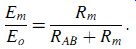
One example of how this technique is applied is in the type of millivoltmeter shown in Figure 2.
This consists of a coil suspended in a fixed magnetic field produced by a permanent magnet.
When an unknown voltage is applied to the coil, the magnetic field due to the current interacts with the fixed field and causes the coil (and a pointer attached to the coil) to turn. If the coil resistance Rcoil is sensitive to temperature, then any environmental input to the system in the form of a temperature change will alter the value of the coil current for a given applied voltage and so alter the pointer output reading. Compensation for this is made by introducing a compensating resistance Rcomp into the circuit, where Rcomp has a temperature coefficient equal in magnitude but opposite in sign to that of the coil. Thus, in response to an increase in temperature, Rcoil increases but Rcomp decreases, and so the total resistance remains approximately the same.
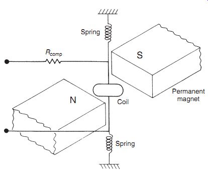
Figure 2
Figure 3
3.4 High-Gain Feedback
The benefit of adding high-gain feedback to many measurement systems is illustrated by considering the case of the voltage-measuring instrument whose block diagram is shown in Figure 3. In this system, unknown voltage Ei is applied to a motor of torque constant Km, and the induced torque turns a pointer against the restraining action of a spring with spring constant Ks. The effect of environmental inputs on the motor and spring constants is represented by variables Dm and Ds. In the absence of environmental inputs, the displacement of the pointer Xo is given by Xo = KmKsEi. However, in the presence of environmental inputs, both Km and Ks change, and the relationship between Xo and Ei can be affected greatly. Therefore, it becomes difficult or impossible to calculate Ei from the measured value of Xo. Consider now what happens if the system is converted into a high-gain, closed-loop one, as shown in Figure 4, by adding an amplifier of gain constant Ka and a feedback device with gain constant Kf. Assume also that the effect of environmental inputs on the values of Ka and Kf are represented by Da and Df. The feedback device feeds back a voltage Eo proportional to the pointer displacement Xo. This is compared with the unknown voltage Ei by a comparator and the error is amplified. Writing down the equations of the system, we have
Thus ...
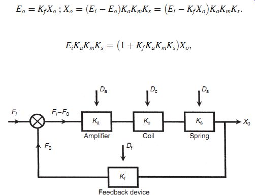
Figure 4
...that is,...
(eqn. 3)
Because Ka is very large (it is a high-gain amplifier), Kf _ Ka _ Km _ Ks >> 1, and Equation ( 3) reduces to
Xo = Ei=Kf :
This is a highly important result because we have reduced the relationship between Xo and Ei to one that involves only Kf. The sensitivity of the gain constants Ka, Km, and Ks to the environmental inputs Da, Dm, and Ds has thereby been rendered irrelevant, and we only have to be concerned with one environmental input, Df. Conveniently, it is usually easy to design a feedback device that is insensitive to environmental inputs: this is much easier than trying to make a motor or spring insensitive. Thus, high-gain feedback techniques are often a very effective way of reducing a measurement system's sensitivity to environmental inputs. However, one potential problem that must be mentioned is that there is a possibility that high-gain feedback will cause instability in the system. Therefore, any application of this method must include careful stability analysis of the system.
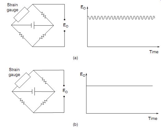
Figure 5
3.5 Signal Filtering
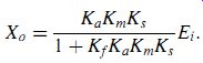
One frequent problem in measurement systems is corruption of the output reading by periodic noise, often at a frequency of 50 Hz caused by pickup through the close proximity of the measurement system to apparatus or current-carrying cables operating on a mains supply.
Periodic noise corruption at higher frequencies is also often introduced by mechanical oscillation or vibration within some component of a measurement system. The amplitude of all such noise components can be substantially attenuated by the inclusion of filtering of an appropriate form in the system, as discussed at greater length in SECTION 6. Band-stop filters can be especially useful where corruption is of one particular known frequency, or, more generally, low-pass filters are employed to attenuate all noise in the frequency range of 50 Hz and above.
Measurement systems with a low-level output, such as a bridge circuit measuring a strain-gauge resistance, are particularly prone to noise, and Figure 5 shows typical corruption of a bridge output by 50-Hz pickup. The beneficial effect of putting a simple passive RC low-pass filter across the output is shown in Figure 5.
3.6 Manual Correction of Output Reading
In the case of errors that are due either to system disturbance during the act of measurement or to environmental changes, a good measurement technician can substantially reduce errors at the output of a measurement system by calculating the effect of such systematic errors and making appropriate correction to the instrument readings. This is not necessarily an easy task and requires all disturbances in the measurement system to be quantified. This procedure is carried out automatically by intelligent instruments.
3.7 Intelligent Instruments
Intelligent instruments contain extra sensors that measure the value of environmental inputs and automatically compensate the value of the output reading. They have the ability to deal very effectively with systematic errors in measurement systems, and errors can be attenuated to very low levels in many cases. A more detailed coverage of intelligent instruments can be found in SECTION 11.
4. Quantification of Systematic Errors
Once all practical steps have been taken to eliminate or reduce the magnitude of systematic errors, the final action required is to estimate the maximum remaining error that may exist in a measurement due to systematic errors. This quantification of the maximum likely systematic error in a measurement requires careful analysis.
4.1 Quantification of Individual Systematic Error Components
The first complication in the quantification of systematic errors is that it is not usually possible to specify an exact value for a component of systematic error, and the quantification has to be in terms of a "best estimate." Once systematic errors have been reduced as far as reasonably possible using the techniques explained in Section 3, a sensible approach to estimate the various kinds of remaining systematic error would be as follows.
Environmental condition errors If a measurement is subject to unpredictable environmental conditions, the usual course of action is to assume midpoint environmental conditions and specify the maximum measurement error as +-x% of the output reading to allow for the maximum expected deviation in environmental conditions away from this midpoint. Of course, this only refers to the case where the environmental conditions remain essentially constant during a period of measurement but vary unpredictably on perhaps a daily basis. If random fluctuations occur over a short period of time from causes such as random draughts of hot or cold air, this is a random error rather than a systematic error that has to be quantified according to the techniques explained in Section 5.
-------
Example 2
The recalibration frequency of a pressure transducer with a range of 0 to 10 bar is set so that it is recalibrated once the measurement error has grown to )1% of the full-scale reading. How can its inaccuracy be expressed in the form of a _x% error in the output reading?
Solution
Just before the instrument is due for recalibration, the measurement error will have grown to +- 0.1 bar (1% of 10 bar). An amount of half this maximum error, that is, 0.05 bar, should be subtracted from all measurements. Having done this, the error just after the instrument has been calibrated will be +-0.05 bar (+-0.5% of full-scale reading) and the error just before the next recalibration will be +-0.05 bar ()0.5% of full-scale reading). Inaccuracy due to calibration error can then be expressed as +-0.05% of full-scale reading.
--------
Calibration errors
All measuring instruments suffer from drift in their characteristics over a period of time. The schedule for recalibration is set so that the frequency at which an instrument is calibrated means that the drift in characteristics by the time just before the instrument is due for recalibration is kept within an acceptable limit. The maximum error just before the instrument is due for recalibration becomes the basis for estimating the maximum likely error. This error due to the instrument being out of calibration is usually in the form of a bias. The best way to express this is to assume some midpoint value of calibration error and compensate all measurements by this midpoint error. The maximum measurement error over the full period of time between when the instrument has just been calibrated and time just before the next calibration is due can then be expressed as _x% of the output reading.
System disturbance errors
Disturbance of the measured system by the act of measurement itself introduces a systematic error that can be quantified for any given set of measurement conditions. However, if the quantity being measured and/or the conditions of measurement can vary, the best approach is to calculate the maximum likely error under worst-case system loading and then to express the likely error as a plus or minus value of half this calculated maximum error, as suggested for calibration errors.
Measurement system loading errors
These have a similar effect to system disturbance errors and are expressed in the form of +-x% of the output reading, where x is half the magnitude of the maximum predicted error under the most adverse loading conditions expected.
4.2 Calculation of Overall Systematic Error
The second complication in the analysis to quantify systematic errors in a measurement system is the fact that the total systemic error in a measurement is often composed of several separate components, for example, measurement system loading, environmental factors, and calibration errors. A worst-case prediction of maximum error would be to simply add up each separate systematic error. For example, if there are three components of systematic error with a magnitude of +-1% each, a worst-case prediction error would be the sum of the separate errors, that is, +-3%. However, it is very unlikely that all components of error would be at their maximum or minimum values simultaneously. The usual course of action is therefore to combine separate sources of systematic error using a root-sum-squares method. Applying this method for n systematic component errors of magnitude +-x1%, +-x2%, +-x3%, +-xn%, the best prediction of likely maximum systematic error by the root-sum-squares method is
Before closing this discussion on quantifying systematic errors, a word of warning must be given about the use of manufacturers' data sheets. When instrument manufacturers provide data sheets with an instrument that they have made, the measurement uncertainty or inaccuracy value quoted in the data sheets is the best estimate that the manufacturer can give about the way that the instrument will perform when it is new, used under specified conditions, and recalibrated at the recommended frequency. Therefore, this can only be a starting point in estimating the measurement accuracy that will be achieved when the instrument is actually used. Many sources of systematic error may apply in a particular measurement situation that are not included in the accuracy calculation in the manufacturer's data sheet, and careful quantification and analysis of all systematic errors are necessary, as described earlier.
------------
Example 3
Three separate sources of systematic error are identified in a measurement system and, after reducing the magnitude of these errors as much as possible, the magnitudes of the three errors are estimated to be System loading: +-1.2% Environmental changes: 0.8% Calibration error: 0.5% Calculate the maximum possible total systematic error and the likely system error by the root-mean-square method.
Solution
The maximum possible system error is +-(1.2 ) 0.8 ) 0.5)% =+-2.5% Applying the root-mean-square method, likely error =_
-------------
5. Sources and Treatment of Random Errors
Random errors in measurements are caused by unpredictable variations in the measurement system. In some books, they are known by the alternative name precision errors. Typical sources of random error are
• measurements taken by human observation of an analogue meter, especially where this involves interpolation between scale points.
• electrical noise.
• random environmental changes, for example, sudden draught of air.
Random errors are usually observed as small perturbations of the measurement either side of the correct value, that is, positive errors and negative errors occur in approximately equal numbers for a series of measurements made of the same constant quantity. Therefore, random errors can largely be eliminated by calculating the average of a number of repeated measurements. Of course, this is only possible if the quantity being measured remains at a constant value during the repeated measurements. This averaging process of repeated measurements can be done automatically by intelligent instruments, as discussed in SECTION 11.
While the process of averaging over a large number of measurements reduces the magnitude of random errors substantially, it would be entirely incorrect to assume that this totally eliminates random errors. This is because the mean of a number of measurements would only be equal to the correct value of the measured quantity if the measurement set contained an infinite number of values. In practice, it is impossible to take an infinite number of measurements. Therefore, in any practical situation, the process of averaging over a finite number of measurements only reduces the magnitude of random error to a small (but nonzero) value. The degree of confidence that the calculated mean value is close to the correct value of the measured quantity can be indicated by calculating the standard deviation or variance of data, these being parameters that describe how the measurements are distributed about the mean value (see Sections 6.1 and 3.6.2). This leads to a more formal quantification of this degree of confidence in terms of the standard error of the mean in Section 6.
6. Statistical Analysis of Measurements Subject to Random Errors
6.1 Mean and Median Values
The average value of a set of measurements of a constant quantity can be expressed as either the mean value or the median value. Historically, the median value was easier for a computer to compute than the mean value because the median computation involves a series of logic operations, whereas the mean computation requires addition and division. Many years ago, a computer performed logic operations much faster than arithmetic operations, and there were computational speed advantages in calculating average values by computing the median rather than the mean. However, computer power increased rapidly to a point where this advantage disappeared many years ago.
As the number of measurements increases, the difference between mean and median values becomes very small. However, the average calculated in terms of the mean value is always slightly closer to the correct value of the measured quantity than the average calculated as the median value for any finite set of measurements. Given the loss of any computational speed advantage because of the massive power of modern-day computers, this means that there is now little argument for calculating average values in terms of the median.
For any set of n measurements x1, x2 ___ xn of a constant quantity, the most likely true value is the mean given by xmean = x1 + x2 )___ xn:

(eqn. 4)
This is valid for all data sets where the measurement errors are distributed equally about the zero error value, that is, where positive errors are balanced in quantity and magnitude by negative errors.
The median is an approximation to the mean that can be written down without having to sum the measurements. The median is the middle value when measurements in the data set are written down in ascending order of magnitude. For a set of n measurements x1, x2 ___ xn of a constant quantity, written down in ascending order of magnitude, the median value is given by xmedian = xn+1=2: (eqn. 5)
Thus, for a set of nine measurements x1, x2 ___ x9 arranged in order of magnitude, the median value is x5. For an even number of measurements, the median value is midway between the two center values, that is, for 10 measurements x1 ___ x10, the median value is given by (x5)x6)/2.
Suppose that the length of a steel bar is measured by a number of different observers and the following set of 11 measurements are recorded (units millimeter). We will call this measurement set A.
398 420 394 416 404 408 400 420 396 413 430 (Measurement set A)
Using Equations ( 4) and ( 5), mean = 409.0 and median = 408. Suppose now that the measurements are taken again using a better measuring rule and with the observers taking more care to produce the following measurement set B:
409 406 402 407 405 404 407 404 407 407 408 (Measurement set B)
For these measurements, mean = 406.0 and median = 407. Which of the two measurement sets, A and B, and the corresponding mean and median values should we have the most confidence in? Intuitively, we can regard measurement set B as being more reliable because the measurements are much closer together. In set A, the spread between the smallest (396) and largest (430) value is 34, while in set B, the spread is only 6.
• Thus, the smaller the spread of the measurements, the more confidence we have in the mean or median value calculated.
Let us now see what happens if we increase the number of measurements by extending measurement set B to 23 measurements. We will call this measurement set C.
409 406 402 407 405 404 407 404 407 407 408 406 410 406 405 408 406 409 406 405 409 406 407
(Measurement set C)
Now, mean = 406.5 and median = 406
• This confirms our earlier statement that the median value tends toward the mean value as the number of measurements increases.
6.2 Standard Deviation and Variance
Expressing the spread of measurements simply as a range between the largest and the smallest value is not, in fact, a very good way of examining how measurement values are distributed about the mean value. A much better way of expressing the distribution is to calculate the variance or standard deviation of the measurements. The starting point for calculating these parameters is to calculate the deviation (error) di of each measurement xi from the mean value xmean in a set of measurements x1,x2, ______xn:
di = xi _ xmean: (eqn. 6)
The variance (Vs) of the set of measurements is defined formally as the mean of the squares of deviations:
(eqn. 7)
The standard deviation (ss) of the set of measurements is defined as the square root of the variance:
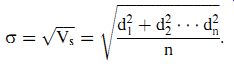
(eqn. 8)
Unfortunately, these formal definitions for the variance and standard deviation of data are made with respect to an infinite population of data values whereas, in all practical situations, we can only have a finite set of measurements. We have made the observation previously that the mean value xm of a finite set of measurements will differ from the true mean m of the theoretical infinite population of measurements that the finite set is part of. This means that there is an error in the mean value xmean used in the calculation of di in Equation ( 6). Because of this, Equations ( 7) and ( 8) give a biased estimate that tends to underestimate the variance and standard deviation of the infinite set of measurements. A better prediction of the variance of the infinite population can be obtained by applying the Bessel correction factor (n/n+1) to the formula for Vs in Equation ( 7):
(eqn. 9)
... where Vs is the variance of the finite set of measurements and V is the variance of the infinite population of measurements.
This leads to a similar better prediction of the standard deviation by taking the square root of the variance in Equation (3.9):
( eqn 10)
6.3 Graphical Data Analysis Techniques-Frequency Distributions
Graphical techniques are a very useful way of analyzing the way in which random measurement errors are distributed. The simplest way of doing this is to draw a histogram, in which bands of equal width across the range of measurement values are defined and the number of measurements within each band is counted. The bands are often given the name data bins. A useful rule for defining the number of bands (bins) is known as the Sturgis rule, which calculates the number of bands as Number of bands = 1 + 3.3 log10 n (),
where n is the number of measurement values.
------------
Example 5
Draw a histogram for the 23 measurements in set C of length measurement data given in Section 5.1.
Solution
For 23 measurements, the recommended number of bands calculated according to the Sturgis rule is 1+3.3 log10 (23)=5.49.
This rounds to five, as the number of bands must be an integer number.
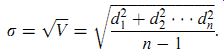
To cover the span of measurements in dataset C with five bands, databands need to be 2 mm wide. The boundaries of these bands must be chosen carefully so that no measurements fall on the boundary between different bands and cause ambiguity about which band to put the min. Because the measurements are integer numbers, this can be accomplished easily by defining the range of the first band as 401.5 to 403.5 and so on. A histogram can now be drawn as in Figure 6 by counting the number of measurements in each band.
In the first band from 401.5 to 403.5, there is just one measurement, so the height of the histogram in this band is 1 unit.
In the next band from 403.5 to 405.5, there are five measurements, so the height of the histogram in this band is 1 = 5 units.
The rest of the histogram is completed in a similar fashion.
When a histogram is drawn using a sufficiently large number of measurements, it will have the characteristic shape shown by truly random data, with symmetry about the mean value of the measurements. However, for a relatively small number of measurements, only approximate symmetry in the histogram can be expected about the mean value. It is a matter of judgment as to whether the shape of a histogram is close enough to symmetry to justify a conclusion that data on which it is based are truly random. It should be noted that the 23 measurements used to draw the histogram in Figure 6 were chosen carefully to produce a symmetrical histogram but exact symmetry would not normally be expected for a measurement data set as small as 23.
As it is the actual value of measurement error that is usually of most concern, it is often more useful to draw a histogram of deviations of measurements from the mean value rather than to draw a histogram of the measurements themselves. The starting point for this is to calculate the deviation of each measurement away from the calculated mean value. Then a histogram of deviations can be drawn by defining deviation bands of equal width and counting the number of deviation values in each band. This histogram has exactly the same shape as the histogram of raw measurements except that scaling of the horizontal axis has to be redefined in terms of the deviation values (these units are shown in parentheses in Figure 6).
Let us now explore what happens to the histogram of deviations as the number of measurements increases. As the number of measurements increases, smaller bands can be defined for the histogram, which retains its basic shape but then consists of a larger number of smaller steps on each side of the peak. In the limit, as the number of measurements approaches infinity, the histogram becomes a smooth curve known as a frequency distribution curve, as shown in Figure 7. The ordinate of this curve is the frequency of occurrence of each deviation value, F(D), and the abscissa is the magnitude of deviation, D.
The symmetry of Figures 6 and 7 about the zero deviation value is very useful for showing graphically that measurement data only have random errors. Although these figures cannot be used to quantify the magnitude and distribution of the errors easily, very similar graphical techniques do achieve this. If the height of the frequency distribution curve is normalized such that the area under it is unity, then the curve in this form is known as a probability curve, and the height F(D) at any particular deviation magnitude D is known as the probability density function (p.d.f.). The condition that the area under the curve is unity can be expressed mathematically as
F(D)dD = 1:
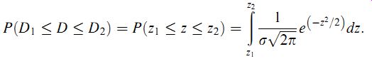
The probability that the error in any one particular measurement lies between two levels D1 and D2 can be calculated by measuring the area under the curve contained between two vertical lines drawn through D1 and D2, as shown by the right-hand hatched area in Figure 7. This can be expressed mathematically as

F(D)dD: ( eqn 11)
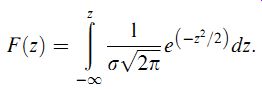
Of particular importance for assessing the maximum error likely in any one measurement is the cumulative distribution function (c.d.f.). This is defined as the probability of observing a value less than or equal to Do and is expressed mathematically as
F(D)dD: ( eqn 12)
Thus, the c.d.f. is the area under the curve to the left of a vertical line drawn through Do, as shown by the left-hand hatched area in Figure 7.
The deviation magnitude Dp corresponding with the peak of the frequency distribution curve (Figure 7) is the value of deviation that has the greatest probability. If the errors are entirely random in nature, then the value of Dp will equal zero. Any nonzero value of Dp indicates systematic errors in data in the form of a bias that is often removable by recalibration.
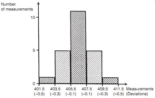
Figure 6
Figure 7
---------------------
6.4 Gaussian ( Normal) Distribution
Measurement sets that only contain random errors usually conform to a distribution with a particular shape that is called Gaussian, although this conformance must always be tested (see the later section headed "Goodness of fit"). The shape of a Gaussian curve is such that the frequency of small deviations from the mean value is much greater than the frequency of large deviations. This coincides with the usual expectation in measurements subject to random errors that the number of measurements with a small error is much larger than the number of measurements with a large error. Alternative names for the Gaussian distribution are normal distribution or bell-shaped distribution. A Gaussian curve is defined formally as a normalized frequency distribution that is symmetrical about the line of zero error and in which the frequency and magnitude of quantities are related by the expression:
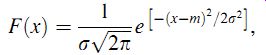
( eqn 13)
where m is the mean value of data set x and the other quantities are as defined before.
Equation ( 13) is particularly useful for analyzing a Gaussian set of measurements and predicting how many measurements lie within some particular defined range. If measurement deviations D are calculated for all measurements such that D = x _ m, then the curve of deviation frequency F(D) plotted against deviation magnitude D is a Gaussian curve known as the error frequency distribution curve. The mathematical relationship between F(D) and D can then be derived by modifying Equation ( 13) to give:
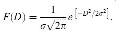
( eqn 14)
The shape of a Gaussian curve is influenced strongly by the value of s, with the width of the curve decreasing as s becomes smaller. As a smaller s corresponds with typical deviations of measurements from the mean value becoming smaller, this confirms the earlier observation that the mean value of a set of measurements gets closer to the true value as s decreases.
If the standard deviation is used as a unit of error, the Gaussian curve can be used to determine the probability that the deviation in any particular measurement in a Gaussian data set is greater than a certain value. By substituting the expression for F(D)in Equation ( 14) into probability Equation ( 11), the probability that the error lies in a band between error levels D1 and D2 can be expressed as ()dD:
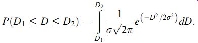
( eqn 15)
Solution of this expression is simplified by the substitution
z = D=s: ( eqn 16)
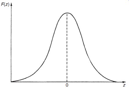
Figure 8
The effect of this is to change the error distribution curve into a new Gaussian distribution that has a standard deviation of one (s =1) and a mean of zero. This new form, shown in Figure 8, is known as a standard Gaussian curve (or sometimes as a z distribution), and the dependent variable is now z instead of D. Equation (3.15) can now be re-expressed as
(eqn 17)
Unfortunately, neither Equation (3.15) nor Equation (3.17) can be solved analytically using tables of standard integrals, and numerical integration provides the only method of solution.
However, in practice, the tedium of numerical integration can be avoided when analyzing data because the standard form of Equation ( 17), and its independence from the particular values of the mean and standard deviation of data, means that standard Gaussian tables that tabulate F(z) for various values of z can be used.
6.5 Standard Gaussian Tables (z Distribution)
Table 1 Error Function Table (Area under a Gaussian Curve or z Distribution)
A standard Gaussian table (sometimes called z distribution), such as that shown in Table 3.1, tabulates the area under the Gaussian curve F(z) for various values of z, where F(z)is given by
=2 ()dz:
( eqn 18)
Thus, F(z) gives the proportion of data values that are less than or equal to z. This proportion is the area under the curve of F(z) against z that is to the left of z. Therefore, the expression given in Equation ( 17) has to be evaluated as [F(z2)_F(z1)]. Study of Table 3.1 shows that F(z) = 0.5 for z = 0. This confirms that, as expected, the number of data values _0 is 50% of the total. This must be so if data only have random errors. It will also be observed that Table 1, in common with most published standard Gaussian tables, only gives F(z) for positive values of z. For negative values of z, we can make use of the following relationship because the frequency distribution curve is normalized:

F _z () = 1 _ Fz (): ( eqn 19)
[F(_z) is the area under the curve to the left of (_z), i.e., it represents the proportion of data values __z.]
6.6 Standard Error of the Mean
The foregoing analysis has examined the way in which measurements with random errors are distributed about the mean value. However, we have already observed that some error exists between the mean value of a finite set of measurements and the true value, that is, averaging a number of measurements will only yield the true value if the number of measurements is infinite. If several subsets are taken from an infinite data population with a Gaussian distribution, then, by the central limit theorem, the means of the subsets will form a Gaussian distribution about the mean of the infinite data set. The standard deviation of mean values of a series of finite sets of measurements relative to the true mean (the mean of the infinite population that the finite set of measurements is drawn from) is defined as the standard error of the mean, a. This is calculated as:
( eqn. 20)
Clearly, a tends toward zero as the number of measurements (n) in the data set expands toward infinity.
The next question is how do we use the standard error of the mean to predict the error between the calculated mean of a finite set of measurements and the mean of the infinite population? In other words, if we use the mean value of a finite set of measurements to predict the true value of the measured quantity, what is the likely error in this prediction? This likely error can only be expressed in probabilistic terms. All we know for certain is the standard deviation of the error, which is expressed as a in Equation (3.20).We also know that a range of _ one standard deviation (i.e., _a) encompasses 68% of the deviations of sample means either side of the true value. Thus we can say that the measurement value obtained by calculating the mean of a set of n measurements, x1, x2, ___ xn, can be expressed as x = xmean _ a with 68% certainty that the magnitude of the error does not exceed |a|. For data set C of length measurements used earlier, n = 23, s = 1.88, and a = 0.39. The length can therefore be expressed as 406.5 +- 0.4 (68% confidence limit).
The problem of expressing the error with 68% certainty is that there is a 32% chance that the error is greater than a. Such a high probability of the error being greater than a may not be acceptable in many situations. If this is the case, we can use the fact that a range of _ two standard deviations, that is, _2a, encompasses 95.4% of the deviations of sample means either side of the true value. Thus, we can express the measurement value as x = xmean _ 2a with 95.4% certainty that the magnitude of the error does not exceed |2a|. This means that there is only a 4.6% chance that the error exceeds 2a. Referring again to set C of length measurements, 2s = 3.76, 2a = 0.78, and the length can be expressed as 406.5 _ 0.8 (95.4% confidence limits).
If we wish to express the maximum error with even greater probability that the value is correct, we could use_3a limits (99.7%confidence). In this case, for length measurements again, 3s = 5.64, 3a = 1.17, and the length should be expressed as 406.5 _ 1.2 (99.7% confidence limits). There is now only a 0.3% chance (3 in 1000) that the error exceeds this value of 1.2.
6.7 Estimation of Random Error in a Single Measurement
In many situations where measurements are subject to random errors, it is not practical to take repeated measurements and find the average value. Also, the averaging process becomes invalid if the measured quantity does not remain at a constant value, as is usually the case when process variables are being measured. Thus, if only one measurement can be made, some means of estimating the likely magnitude of error in it is required. The normal approach to this is to calculate the error within 95%confidence limits, that is, to calculate the value of deviation D such that 95%of the area under the probability curve lies within limits of _D. These limits correspond to a deviation of +-1.96s. Thus, it is necessary to maintain the measured quantity at a constant value while a number of measurements are taken in order to create a reference measurement set from which s can be calculated. Subsequently, the maximum likely deviation in a single measurement can be expressed as Deviation =_1.96s. However, this only expresses the maximum likely deviation of the measurement from the calculated mean of the reference measurement set, which is not the true value as observed earlier. Thus the calculated value for the standard error of the mean has to be added to the likely maximum deviation value. To be consistent, this should be expressed to the same 95% confidence limits. Thus, the maximum likely error in a single measurement can be expressed as

( eqn 21)
Before leaving this matter, it must be emphasized that the maximum error specified for a measurement is only specified for the confidence limits defined. Thus, if the maximum error is specified as _1% with 95% confidence limits, this means that there is still 1 chance in 20 that the error will exceed +-1%.
----------------
Example 7
Suppose that a standard mass is measured 30 times with the same instrument to create a reference data set, and the calculated values of s and a are s = 0.46 and a = 0.08. If the instrument is then used to measure an unknown mass and the reading is 105.6 kg, how should the mass value be expressed?
Solution
Using Equation ( 21), 1.96(s ) a) = 1.06.
The mass value should therefore be expressed as 105.6 _ 1.1 kg.
----------------
6.8 Distribution of Manufacturing Tolerances
Many aspects of manufacturing processes are subject to random variations caused by factors similar to those that cause random errors in measurements. In most cases, these random variations in manufacturing, which are known as tolerances, fit a Gaussian distribution, and the previous analysis of random measurement errors can be applied to analyze the distribution of these variations in manufacturing parameters.
6.9 Chi-Squared (x2) Distribution
We have already observed the fact that, if we calculate the mean value of successive sets of samples of N measurements, the means of those samples form a Gaussian distribution about the true value of the measured quantity (the true value being the mean of the infinite data set that the set of samples are part of). The standard deviation of the distribution of the mean values was quantified as the standard error of the mean.
It is also useful for many purposes to look at distribution of the variance of successive sets of samples of N measurements that form part of a Gaussian distribution. This is expressed as the chi-squared distribution F(w2 ), where w2 is given by w^2 = ksx 2
=s2 , (eqn. 22) where sx 2 is the variance of a sample of N measurements and s2 is the variance of the infinite data set that sets of N samples are part of. k is a constant known as the number of degrees of freedom and is equal to (N+1).
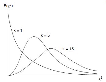
Figure 10
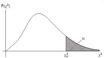
Figure 11
The shape of the w2 distribution depends on the value of k, with typical shapes being shown in Figure 10. The area under the w2 distribution curve is unity but, unlike the Gaussian distribution, the w2 distribution is not symmetrical. However, it tends toward the symmetrical shape of a Gaussian distribution as k becomes very large.
The w2 distribution expresses the expected variation due to random chance of the variance of a sample away from the variance of the infinite population that the sample is part of. The magnitude of this expected variation depends on what level of "random chance" we set. The level of random chance is normally expressed as a level of significance, which is usually denoted by the symbol a. Referring to the w2 distribution shown in Figure 11,value w2 a denotes the w2 value to the left of which lies 100(1+a)% of the area under the w2 distribution curve. Thus, the area of the curve to the right of w2 a is a and that to the left is (1+a).
Numerical values for w2 are obtained from tables that express the value of w2 for various degrees of freedom k and for various levels of significance a. Published tables differ in the number of degrees of freedom and the number of levels of significance covered. A typical table is shown as Table 2.
One major use of the w2 distribution is to predict the variance s2 of an infinite data set, given the measured variance sx 2 of a sample of N measurements drawn from the infinite population.
The boundaries of the range of w2 values expected for a particular level of significance a can be expressed by the probability expression:
( eqn 23)
To put this in simpler terms, we are saying that there is a probability of (1_a)% that w2 lies within the range bounded by w2 1+a=2 and w2 a=2 for a level of significance of a. For example, for a level of significance a = 0.5, there is a 95%probability (95%confidence level) that w2 lies between w2
0:975 and w2
0:025.
Substituting into Equation ( 23) using the expression for w2 given in Equation ( 22):
This can be expressed in an alternative but equivalent form by inverting the terms and changing the "_" relationships to " " ones:
Now multiplying the expression through by ksx 2 gives the following expression for the boundaries of the variance s2:
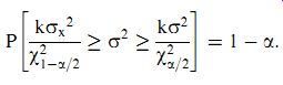
(eqn 24)
The thing that is immediately evident in this solution is that the range within which the true variance and standard deviation lies is very wide. This is a consequence of the relatively small number of measurements (10) in the sample. It is therefore highly desirable wherever possible to use a considerably larger sample when making predictions of the true variance and standard deviation of some measured quantity.
The solution to Example 3.10 shows that, as expected, the width of the estimated range in which the true value of the standard deviation lies gets wider as we increase the confidence level from 90 to 99%. It is also interesting to compare the results in Examples 9 and 10 for the same confidence level of 95%. The ratio between maximum and minimum values of estimated variance is much greater for the 10 samples in Example 9 compared with the 25 samples in Example 10. This shows the benefit of having a larger sample size when predicting the variance of the whole population that the sample is drawn from.
6.10 Goodness of Fit to a Gaussian Distribution
All of the analysis of random deviations presented so far only applies when data being analyzed belong to a Gaussian distribution. Hence, the degree to which a set of data fits a Gaussian distribution should always be tested before any analysis is carried out. This test can be carried out in one of three ways:
(a) Inspecting the shape of the histogram: The simplest way to test for Gaussian distribution of data is to plot a histogram and look for a "bell shape" of the form shown earlier in Figure 6. Deciding whether the histogram confirms a Gaussian distribution is a matter of judgment. For a Gaussian distribution, there must always be approximate symmetry about the line through the center of the histogram, the highest point of the histogram must always coincide with this line of symmetry, and the histogram must get progressively smaller either side of this point. However, because the histogram can only be drawn with a finite set of measurements, some deviation from the perfect shape of histogram as described previously is to be expected even if data really are Gaussian.
(b) Using a normal probability plot: A normal probability plot involves dividing data values into a number of ranges and plotting the cumulative probability of summed data frequencies against data values on special graph paper.* This line should be a straight line if the data distribution is Gaussian. However, careful judgment is required, as only a finite number of data values can be used and therefore the line drawn will not be entirely straight even if the distribution is Gaussian. Considerable experience is needed to judge whether the line is straight enough to indicate a Gaussian distribution. This will be easier to understand if data in measurement set C are used as an example. Using the same five ranges as used to draw the histogram, the following table is first drawn:
The normal probability plot drawn from this table is shown in Figure 12. This is sufficiently straight to indicate that data in measurement set C are Gaussian.
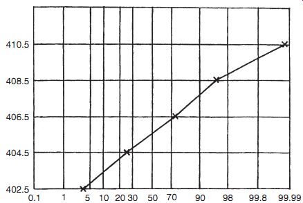
Figure 12
(c) The w2 test: The w2 distribution provides a more formal method for testing whether data follow a Gaussian distribution. The principle of the w2 test is to divide data into p equal width bins and to count the number of measurements ni in each bin, using exactly the same procedure as done to draw a histogram. The expected number of measurements ni 0 in each bin for a Gaussian distribution is also calculated. Before proceeding any further, a check must be made at this stage to confirm that at least 80% of the bins have a data count greater than a minimum number for both ni and ni 0. We will apply a minimum number of four, although some statisticians use the smaller minimum of three and some use a larger minimum of five. If this check reveals that too many bins have data counts less than the minimum number, it is necessary to reduce the number of bins by redefining their widths. The test for at least 80% of the bins exceeding the minimum number then has to be reapplied. Once the data count in the bins is satisfactory, a w2 value is calculated for data according to the following formula:
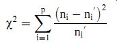
( eqn 25)
The w2 test then examines whether the calculated value of w2 is greater than would be expected for a Gaussian distribution according to some specified level of chance.
This involves reading off the expected value from the w2 distribution table (Table 2) for the specified confidence level and comparing this expected value with that calculated in Equation ( 25). This procedure will become clearer if we work through an example.
6.11 Rogue Data Points (Data Outliers)
In a set of measurements subject to random error, measurements with a very large error sometimes occur at random and unpredictable times, where the magnitude of the error is much larger than could reasonably be attributed to the expected random variations in measurement value. These are often called rogue data points or data outliers. Sources of such abnormal error include sudden transient voltage surges on the main power supply and incorrect recording of data (e.g., writing down 146.1 when the actual measured value was 164.1). It is accepted practice in such cases to discard these rogue measurements, and a threshold level of a +-3s deviation is often used to determine what should be discarded. It is rare for measurement errors to exceed +-3s limits when only normal random effects are affecting the measured value.
While the aforementioned represents a reasonable theoretical approach to identifying and eliminating rogue data points, the practical implementation of such a procedure needs to be done with care. The main practical difficulty that exists in dealing with rogue data points is in establishing what the expected standard deviation of the measurements is.
When a new set of measurements is being taken where the expected standard deviation is not known, the possibility exists that a rogue data point exists within the measurements.
Simply applying a computer program to the measurements to calculate the standard deviation will produce an erroneous result because the calculated value will be biased by the rogue data point. The simplest way to overcome this difficulty is to plot a histogram of any new set of measurements and examine this manually to spot any data outliers. If no outliers are apparent, the standard deviation can be calculated and then used in a _3s threshold against which to test all future measurements. However, if this initial data histogram shows up any outliers, these should be excluded from the calculation of the standard deviation.
It is interesting at this point to return to the problem of ensuring that there are no outliers in the set of data used to calculate the standard deviation of data and hence the threshold for rejecting outliers. We have suggested that a histogram of some initial measurements be drawn and examined for outliers. What would happen if the set of data given earlier in Example 13 was the initial data set that was examined for outliers by drawing a histogram? What would happen if we did not spot the outlier of 4.59? This question can be answered by looking at the effect on the calculated value of standard deviation if this rogue data point of 4.59 is included in the calculation. The standard deviation calculated over the 19 values, excluding the 4.59 measurement, is 0.052. The standard deviation calculated over the 20 values, including the 4.59 measurement, is 0.063 and the mean data value is changed to 4.42. This gives a 3s threshold of 0.19, and the boundaries for the +-3s threshold operation are now 4.23 and 4.61. This does not exclude the data value of 4.59, which we identified previously as a being a rogue data point! This confirms the necessity of looking carefully at the initial set of data used to calculate the thresholds for rejection of the rogue data point to ensure that initial data do not contain any rogue data points. If drawing and examining a histogram do not clearly show that there are no rogue data points in the "reference" set of data, it is worth taking another set of measurements to see whether a reference set of data can be obtained that is more clearly free of rogue data points.
----
Example 13
A set of measurements is made with a new pressure transducer. Inspection of a histogram of the first 20 measurements does not show any data outliers. The standard deviation of the measurements is calculated as 0.05 bar after this check for data outliers, and the mean value is calculated as 4.41. Following this, the following further set of measurements is obtained:
4.35 4.46 4.39 4.34 4.41 4.52 4.44 4.37 4.41 4.33 4.39 4.47 4.42 4.59 4.45 4.38 4.43 4.36 4.48 4.45
Use the +-3s threshold to determine whether there are any rogue data points in the measurement set.
Solution Because the calculated s value for a set of "good" measurements is given as 0.05, the +-3s threshold is +-0.15. With a mean data value of 4.41, the threshold for rogue data points is values below 4.26 (mean value minus 3s) or above 4.56 (mean value plue 3s).
Looking at the set of measurements, we observe that the measurement of 4.59 is outside the +-3s threshold, indicating that this is a rogue data point.
---------------
6.12 Student t Distribution
When the number of measurements of a quantity is particularly small (less than about 30 samples) and statistical analysis of the distribution of error values is required, the possible deviation of the mean of measurements from the true measurement value (the mean of the infinite population that the sample is part of) may be significantly greater than is suggested by analysis based on a z distribution. In response to this, a statistician called William Gosset developed an alternative distribution function that gives a more accurate prediction of the error distribution when the number of samples is small. He published this under the pseudonym "Student" and the distribution is commonly called student t distribution. It should be noted that t distribution has the same requirement as the z distribution in terms of the necessity for data to belong to a Gaussian distribution.
The student t variable expresses the difference between the mean of a small sample xmean () and the population mean (m) in terms of the following ratio:
t = j error in mean j standard error of the mean: (eqn. 26)
Because we do not know the exact value of s, we have to use the best approximation to s that we have, which is the standard deviation of the sample, sx. Substituting this value for s in Equation ( 26) gives
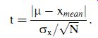
( eqn 27)
Note that the modulus operation (| ___ |) on the error in the mean in Equations ( 26) and ( 27) means that t is always positive.
The shape of the probability distribution curve F(t) of the t variable varies according to the value of the number of degrees of freedom, k (= N _ 1), with typical curves being shown in Figure 13. Ask!1, F(t)!F(z), that is, the distribution becomes a standard Gaussian one. For values of k<1, the curve of F(t) against t is both narrower and less high in the center than a standard Gaussian curve, but has the same properties of symmetry about t = 0 and a total area under the curve of unity.
In a similar way to z distribution, the probability that t will lie between two values t1 and t2 is given by the area under the F(t) curve between t1 and t2. The t distribution is published in the form of a standard table (see Table 3.3) that gives values of the area under the curve a for various values of k, where
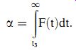
( eqn 28)
The area a is shown in Figure 14. a corresponds to the probability that t will have a value greater than t3 to some specified confidence level. Because the total area under the F(t) curve is unity, there is also a probability of (1+a) that t will have a value less than t3. Thus, for a value a=0.05, there is a 95% probability (i.e., a 95% confidence level) that t < t3.
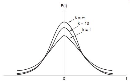
Figure 13
Table 3 -- Distribution
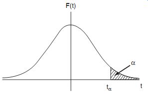
Figure 14
Because of the symmetry of t distribution, a is also given by
( 29) as shown in Figure 15. Here, a corresponds to the probability that t will have a value less than +-t3, with a probability of (1+a) that t will have a value greater than +-t3.
Equations ( 28) and ( 29) can be combined to express the probability (1+a) that t lies between two values +-t4 and + t4. In this case, a is the sum of two areas of a/2 as shown in Figure 16. These two areas can be represented mathematically as
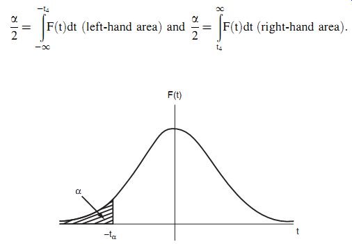
Figure 15
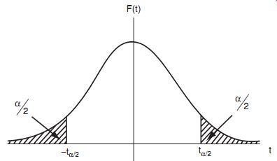
Figure 16
The values of t4 can be found in any t distribution table, such as Table 3.
Referring back to Equation ( 27), this can be expressed in the form:
Hence, upper and lower bounds on the expected value of the population mean m (the true value of x) can be expressed as

( eqn 30)
Out of interest, let us examine what would have happened if we had calculated the error bounds on m using standard Gaussian (z-distribution) tables. For 95% confidence, the maximum error is given as
+- 1:96s= N p , that is, +-0.96, which rounds to +-1.0 mm, meaning the mean internal diameter is given as 105.4 + 1.0 mm. The effect of using t distribution instead of z distribution clearly expands the magnitude of the likely error in the mean value to compensate for the fact that our calculations are based on a relatively small number of measurements.
7. Aggregation of Measurement System Errors
Errors in measurement systems often arise from two or more different sources, and these must be aggregated in the correct way in order to obtain a prediction of the total likely error in output readings from the measurement system. Two different forms of aggregation are required: (1) a single measurement component may have both systematic and random errors and (2) a measurement system may consist of several measurement components that each have separate errors.
7.1 Combined Effect of Systematic and Random Errors
If a measurement is affected by both systematic and random errors that are quantified as _x (systematic errors) and _y (random errors), some means of expressing the combined effect of both types of errors is needed. One way of expressing the combined error would be to sum the two separate components of error, that is, to say that the total possible error is e =_(x ) y). However, a more usual course of action is to express the likely maximum error as

( eqn 31)
It can be shown (ANSI/ASME, 1985) that this is the best expression for the error statistically, as it takes into account the reasonable assumption that the systematic and random errors are independent and so it is unlikely that both will be at their maximum or minimum value simultaneously.
7.2 Aggregation of Errors from Separate Measurement System Components
A measurement system often consists of several separate components, each of which is subject to errors. Therefore, what remains to be investigated is how errors associated with each measurement system component combine together so that a total error calculation can be made for the complete measurement system. All four mathematical operations of addition, subtraction, multiplication, and division may be performed on measurements derived from different instruments/transducers in a measurement system. Appropriate techniques for the various situations that arise are covered later.
Error in a sum
If the two outputs y and z of separate measurement system components are to be added together, we can write the sum as S = y ) z. If the maximum errors in y and z are _ay and
_bz, respectively, we can express the maximum and minimum possible values of S as Smax = y ) ay ()) z ) bz) ; Smin = y _ ay ()) z _ bz () ;or S = y ) z _ ay ) bz (): ( This relationship for S is not convenient because in this form the error term cannot be expressed as a fraction or percentage of the calculated value for S. Fortunately, statistical analysis can be applied (see Topping, 1962) that expresses S in an alternative form such that the most probable maximum error in S is represented by a quantity e, where e is calculated in terms of the absolute errors as

(eqn. 32)
Thus S = (y ) z) _ e. This can be expressed in the alternative form:
S = y ) z () 1 _ f (), ( 3:33) where f = e/(y ) z).
It should be noted that Equations ( 32) and ( 33) are only valid provided that the measurements are uncorrelated (i.e., each measurement is entirely independent of the others).
Error in a difference If the two outputs y and z of separate measurement systems are to be subtracted from one another, and the possible errors are _ay and _bz, then the difference S can be expressed (using statistical analysis as for calculating the error in a sum and assuming that the measurements are uncorrelated) as
S = y _ z ()_ e or S = y _ z () 1 _ f (), where e is calculated as in Equation ( 32) and f = e/(y _ z).
This example illustrates very poignantly the relatively large error that can arise when calculations are made based on the difference between two measurements.
Error in a product
If outputs y and z of two measurement system components are multiplied together, the product can be written as P = yz. If the possible error in y is _ay and in z is _bz, then the maximum and minimum values possible in P can be written as
Pmax = y ) ay () z ) bz ()= yz ) ayz ) byz ) aybz ; Pmin = y _ ay () z _ bz ()
= yz _ ayz _ byz ) aybz:
For typical measurement system components with output errors of up to 1 or 2% in magnitude, both a and b are very much less than one in magnitude and thus terms in aybz are negligible compared with other terms. Therefore, we have Pmax=yz(1)a)b); Pmin=yz(1_a_b).
Thus the maximum error in product P is _(a ) b).While this expresses the maximum possible error in P, it tends to overestimate the likely maximum error, as it is very unlikely that the errors in y and z will both be at the maximum or minimum value at the same time. A statistically better estimate of the likely maximum error e in product P, provided that the measurements are uncorrelated, is given by Topping (1962):

(eqn. 34)
Note that in the case of multiplicative errors, e is calculated in terms of fractional errors in y and z (as opposed to absolute error values used in calculating additive errors).
Error in a quotient
If the output measurement y of one system component with possible error _ay is divided by the output measurement z of another system component with possible error _bz, then the maximum
Thus the maximum error in the quotient is _(a ) b). However, using the same argument as made earlier for the product of measurements, a statistically better estimate (see Topping, 1962) of the likely maximum error in the quotient Q, provided that the measurements are uncorrelated, is that given in Equation ( 34).
7.3 Total Error When Combining Multiple Measurements
The final case to be covered is where the final measurement is calculated from several measurements that are combined together in a way that involves more than one type of arithmetic operation. For example, the density of a rectangular-sided solid block of material can be calculated from measurements of its mass divided by the product of measurements of its length, height, and width. Because errors involved in each stage of arithmetic are cumulative, the total measurement error can be calculated by adding together the two error values associated with the two multiplication stages involved in calculating the volume and then calculating the error in the final arithmetic operation when the mass is divided by the volume.
8. Summary
This SECTION introduced the subject of measurement uncertainty, and the length of the SECTION gives testimony to the great importance attached to this subject. Measurement errors are a fact of life and, although we can do much to reduce the magnitude of errors, we can never reduce errors entirely to zero. We started the SECTION off by noting that measurement uncertainty comes in two distinct forms, known respectively as systematic error and random error. We learned that the nature of systematic errors was such that the effect on a measurement reading was to make it either consistently greater than or consistently less than the true value of the measured quantity. Random errors, however, are entirely random in nature, such that successive measurements of a constant quantity are randomly both greater than and less than the true value of the measured quantity.
In our subsequent study of systematic measurement errors, we first examined all the sources of this kind of error. Following this, we looked at all the techniques available for reducing the magnitude of systematic errors arising from the various error sources identified. Finally, we examined ways of quantifying the remaining systemic measurement error after all reasonable means of reducing error magnitude had been applied.
Our study of random measurement errors also started off by studying typical sources of these.
We observed that the nature of random errors means that we can get close to the correct value of the measured quantity by averaging over a number of measurements, although we noted that we could never actually get to the correct value unless we achieved the impossible task of having an infinite number of measurements to average over. We found that how close we get to the correct value depends on how many measurements we average over and how widely the measurements are spread. We then examined the two alternative ways of calculating an average in terms of the mean and median value of a set of measurements. Following this, we looked at ways of expressing the spread of measurements about the mean/median value. This led to the formal mathematical quantification of spread in terms of standard deviation and variance. We then started to look at graphical ways of expressing the spread. Initially, we considered representations of spread as a histogram and then went on to show how histograms expand into frequency distributions in the form of a smooth curve. We found that truly random data are described by a particular form of frequency distribution known as Gaussian (or normal).We introduced the z variable and saw how this can be used to estimate the number of measurements in a set of measurements that have an error magnitude between two specified values. Following this, we looked at the implications of the fact that we can only ever have a finite number of measurements. We saw that a variable called the standard error of the mean could be calculated that estimates the difference between the mean value of a finite set of measurements and the true value of the measured quantity (the mean of an infinite data set). We went on to look at how this was useful in estimating the likely error in a single measurement subject to random errors in the situation where it is not possible to average over a number of measurements. As an aside, we then went on to look at how the z variable was useful in analyzing tolerances of manufactured components subject to random variations in a parallel way to the analysis of measurements subject to random variations. Following this, we went onto look at w2 distribution. This can be used to quantify the variation in the variance of a finite set of measurements with respect to the variance of the infinite set that the finite set is part of. Up until this point in the SECTION, all analysis of random errors assumed that the measurement set fitted a Gaussian distribution. However, this assumption must always be justified by applying goodness of fit tests, so these were explained in the following section, where we saw that a w2 test is the most rigorous test available for goodness of fit. A particular problem that can affect the analysis of random errors adversely is the presence of rogue data points (data outliers) in measurement data. These were considered, and the conditions under which they can justifiably be excluded from the analyzed data set were explored. Finally, we saw that yet another problem that can affect the analysis of random errors is where the measurement set only has a small number of values. In this case, calculations based on z distribution are inaccurate, and we explored the use of a better distribution called t distribution.
The SECTION ended with looking at how the effects of different measurement errors are aggregated together to predict the total error in a measurement system. This process was considered in two parts. First, we looked at how systematic and random error magnitudes can be combined together in an optimal way that best predicts the likely total error in a particular measurement. Second, we looked at situations where two or more measurements of different quantities are combined together to give a composite measurement value and looked at the best way of dealing with each of the four arithmetic operations that can be carried out on different measurement components.
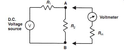
Figure 17
9. Problems
1. Explain the difference between systematic and random errors. What are the typical sources of these two types of errors? 3.2. In what ways can the act of measurement cause a disturbance in the system being measured? 3.3. In the circuit shown in Figure 17, the resistor values are given by R1 = 1000 Ohm ; R2 = 1000 Ohm ;V = 20 volts. The voltage across AB (i.e., across R2) is measured by a voltmeter whose internal resistance is given by Rm = 9500 Ohm.
(a) What will be the reading on the voltmeter? (b) What would the voltage across AB be if the voltmeter was not loading the circuit (i.e., if Rm = infinity)? (c) What is the measurement error due to the loading effect of the voltmeter?
4. Suppose that the components in the circuit shown in Figure 1a have the following values:
R1 = 330 O; R2 = 1000 O; R3 = 1200 O; R4 = 220 O;R5 = 270 O:
If the instrument measuring the output voltage across AB has a resistance of 5000 O, what is the measurement error caused by the loading effect of this instrument?
5. (a) Explain what is meant by the term "modifying inputs." (b) Explain briefly what measures can be taken to reduce or eliminate the effect of modifying inputs.
6. Instruments are normally calibrated and their characteristics defined for particular standard ambient conditions. What procedures are normally taken to avoid measurement errors when using instruments subjected to changing ambient conditions?
7. The voltage across a resistance R5 in the circuit of Figure 18 is to be measured by a voltmeter connected across it.
(a) If the voltmeter has an internal resistance (Rm) of 4750 O, what is the measurement error? (b) What value would the voltmeter internal resistance need to be in order to reduce the measurement error to 1%? 8. In the circuit shown in Figure 19, the current flowing between A and B is measured by an ammeter whose internal resistance is 100 O. What is the measurement error caused by the resistance of the measuring instrument?
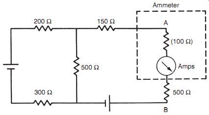
Figure 19
9. What steps can be taken to reduce the effect of environmental inputs in measurement systems?
10. (a) Explain why a voltmeter never reads exactly the correct value when it is applied to an electrical circuit to measure the voltage between two points.
(b) For the circuit shown in Figure 17, show that the voltage Em measured across points AB by the voltmeter is related to the true voltage Eo by the following expression:
(c) If the parameters in Figure 17 have the following values, R1= 500 Ohm; R2 = 500 Ohm; Rm = 4750 Ohm, calculate the percentage error in the voltage value measured across points AB by the voltmeter.
11. The output of a potentiometer is measured by a voltmeter having resistance Rm,as shown in Figure 20. Rt is the resistance of the total length Xt of the potentiometer, and Ri is the resistance between the wiper and common point C for a general wiper position Xi. Show that the measurement error due to the resistance, Rm, of the measuring instrument is given by
Hence show that the maximum error occurs when Xi is approximately equal to 2Xt/3.
(Hint: differentiate the error expression with respect to Ri and set to 0. Note that maximum error does not occur exactly at Xi = 2Xt/3, but this value is very close to the position where the maximum error occurs.)
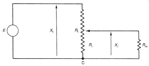
Figure 20
12. In a survey of 15 owners of a certain model of car, the following values for average fuel consumption were reported:
25.5 30.3 31.1 29.6 32.4 39.4 28.9 30.0 33.3 31.4 29.5 30.5 31.7 33.0 29.2
Calculate mean value, median value, and standard deviation of the data set.
13. The following 10 measurements of the freezing point of aluminum were made using a platinum/rhodium thermocouple:
658.2 659.8 661.7 662.1 659.3 660.5 657.9 662.4 659.6 662.2
Find (a) median, (b)mean, (c) standard deviation, and (d) variance of the measurements.
14. The following 25 measurements were taken of the thickness of steel emerging from a rolling mill:
97 3.99 4.04 4.00 3.98 4.03 4.00 3.98 3.99 3.96 4.02 3.99 4.01 3.97 4.02 3.99 3.95 4.03 4.01 4.05 3.98 4.00 4.04 3.98 4.02
Find (a) median, (b)mean, (c) standard deviation, and (d) variance of the measurements.
15. The following 10 measurements were made of output voltage from a high-gain amplifier contaminated due to noise fluctuations:
1.53, 1.57, 1.54, 1.54 ,1.50, 1.51, 1.55, 1.54, 1.56, 1.53
Determine the mean value and standard deviation. Hence, estimate the accuracy to which the mean value is determined from these 10measurements. If 1000measurements were taken, instead of 10, but s remained the same, by how much would the accuracy of the calculated mean value be improved?
16. The following measurements were taken with an analogue meter of current flowing in a circuit (the circuit was in steady state and therefore, although measurements varied due to random errors, the current flowing was actually constant):
21.5, 22.1, 21.3, 21.7, 22.0, 22.2, 21.8, 21.4, 21.9, 22.1 mA
Calculate mean value, deviations from the mean, and standard deviation.
17. Using the measurement data given in Problem 14, draw a histogram of errors (use error bands 0.03 units wide, i.e., the center band will be from -0.015 to +0.015).
18. (a) What do you understand by the term probability density function? (b) Write down an expression for a Gaussian probability density function of given mean value m and standard deviation s and show how you would obtain the best estimates of these two quantities from a sample of population n.
19. Measurements in a data set are subject to random errors, but it is known that the data set fits a Gaussian distribution. Use standard Gaussian tables to determine the percentage of measurements that lie within the boundaries of +-1.5s, where s is the standard deviation of the measurements.
20. Measurements in a data set are subject to random errors, but it is known that the data set fits a Gaussian distribution. Use error function tables to determine the value of x required such that 95%of the measurements lie within the boundaries of_xs, where s is the standard deviation of the measurements.
21. By applying error function tables for mean and standard deviation values calculated in Problem 14, estimate (a) How many measurements are <4.00? (b) How many measurements are <3.95? (c) How many measurements are between 3.98 and 4.02? Check your answers against real data.
22. The resolution of the instrument referred to in Problem 14 is clearly 0.01.
Because of the way in which error tables are presented, estimations of the number of measurements in a particular error band are likely to be closer to the real number if boundaries of the error band are chosen to be between measurement values. In part c of Problem 21, values >3.98 are subtracted from values >4.02, thus excluding measurements equal to 3.98. Test this hypothesis out by estimating:
(a) How many measurements are <3.995?
(b) How many measurements are <3.955?
(c) How many measurements are between 3.975 and 4.025?
Check your answers against real data.
23. Measurements in a data set are subject to random errors, but it is known that the data set fits a Gaussian distribution. Use error function tables to determine the percentage of measurements that lie within the boundaries of +-2s , where s is the standard deviation of the measurements.
24. A silicon-integrated circuit chip contains 5000 ostensibly identical transistors.
Measurements are made of the current gain of each transistor. Measurements have a mean of 20.0 and a standard deviation of 1.5. The probability distribution of the measurements is Gaussian.
(a) Write down an expression for the number of transistors on the chip that have a current gain between 19.5 and 20.5.
(b) Show that this number of transistors with a current gain between 19.5 and 20.5 is approximately 1300.
(c) Calculate the number of transistors that have a current gain of 17 or more (this is the minimum current gain necessary for a transistor to be able to drive the succeeding stage of the circuit in which the chip is used).
25. In a particular manufacturing process, bricks are produced in batches of 10,000.
Because of random variations in the manufacturing process, random errors occur in the target length of the bricks produced. If the bricks have a mean length of 200 mm with a standard deviation of 20 mm, show how the error function tables supplied can be used to calculate the following:
(a) number of bricks with a length between 198 and 202 mm.
(b) number of bricks with a length greater than 170 mm.
26. The temperature-controlled environment in a hospital intensive care unit is monitored by an intelligent instrument that measures temperature every minute and calculates the mean and standard deviation of the measurements. If the mean is 75 C and the standard deviation is 2.15, (a) What percentage of the time is the temperature less than 70 C? (b) What percentage of the time is the temperature between 73 and 77 C?
27. Calculate the standard error of the mean for measurements given in Problem 13.
Hence, express the melting point of aluminum together with the possible error in the value expressed.
28. The thickness of a set of gaskets varies because of random manufacturing disturbances, but thickness values measured belong to a Gaussian distribution. If the mean thickness is 3 mm and the standard deviation is 0.25, calculate the percentage of gaskets that have a thickness greater than 2.5 mm.
29. If the measured variance of 25 samples of bread cakes taken from a large batch is 4.85 grams, calculate the true variance of the mass for a whole batch of bread cakes to a 95% significance level.
30. Calculate true standard deviation of the diameter of a large batch of tires to a confidence level of 99% if the measured standard deviation in the diameter for a sample of 30 tires is 0.63 cm.
31. One hundred fifty measurements are taken of the thickness of a coil of rolled steel sheet measured at approximately equidistant points along the center line of its length.
Measurements have a mean value of 11.291 mm and a standard deviation of 0.263 mm.
The smallest and largest measurements in the sample are 10.73 and 11.89 mm.
Measurements are divided into eight data bins with boundaries at 10.695, 10.845, 10.995, 11.145, 11.295, 11.445, 11.595, 11.745, and 11.895. The first bin, containing measurements between 10,695 and 10.845, has eight measurements in it, and the count of measurements in the following successive bins is 12, 21, 34, 31, 25, 14, and 5. Apply the w2 test to see whether the measurements fit a Gaussian distribution to a 95% confidence level.
32. The temperature in a furnace is regulated by a control system that aims to keep the temperature close to 800 C. The temperature is measured every minute over a 2-hour period, during which time the minimum and maximum temperatures measured are 782 and 819 C. Analysis of the 120 measurements shows a mean value of 800.3 C and a standard deviation of 7.58 C. Measurements are divided into eight data bins of 5 C width with boundaries at 780.5, 785.5, 790.5, 795.5, 800.5, 805.5, 810.5, 815.5, and 820.5. The measurement count in bin one from 780.5 to 785.5 C was 3, and the count in the other successive bins was 8, 21, 30, 28, 19, 9, and 2. Apply the w2 test to see whether the measurements fit a Gaussian distribution to (a) a 90% confidence level and (b) a 95%confidence level (think carefully about whether the w2 test will be reliable for the measurement counts observed and whether there needs to be any change in the number of data bins used for the w2 test).
33. The volume contained in each sample of 10 bottles of expensive perfume is measured.
If the mean volume of the sample measurements is 100.5 ml with a standard deviation of 0.64 ml, calculate the upper and lower bounds to a confidence level of 95% of the mean value of the whole batch of perfume from which the 10 samples were taken.
34. A 3-volt d.c. power source required for a circuit is obtained by connecting together two 1.5-volt batteries in series. If the error in the voltage output of each battery is specified as +-1%, calculate the likely maximum error in the 3-volt power source that they make up.
35. A temperature measurement system consists of a thermocouple whose amplified output is measured by a voltmeter. The output relationship for the thermocouple is approximately linear over the temperature range of interest. The e.m.f./temp relationship of the thermocouple has a possible error of +-1%, the amplifier gain value has a possible error of +-0.5%, and the voltmeter has a possible error of +-2%.
What is the possible error in the measured temperature?
36. A pressure measurement system consists of a monolithic piezoresistive pressure transducer and a bridge circuit to measure the resistance change of the transducer. The resistance (R) of the transducer is related to pressure (P) according to R = K1 P and the output of the bridge circuit (V) is related to resistance (R)by V =K2 R. Thus, the output voltage is related to pressure according to V = K1 K2 P. If the maximum error in K1 is +-2%, the maximum error in K2 is +-1.5%, and the voltmeter itself has a maximum measurement error of +-1%, what is the likely maximum error in the pressure measurement?
37. A requirement for a resistance of 1220 O in a circuit is satisfied by connecting together resistances of 1000 and 220 Ohm in series. If each resistance has a tolerance of +-5%, what is the likely tolerance in the total resistance?
38. In order to calculate the heat loss through the wall of a building, it is necessary to know the temperature difference between inside and outside walls. Temperatures of 5 and 20 C are measured on each side of the wall by mercury-in-glass thermometers with a range of 0 to +50 C and a quoted inaccuracy of +-1% of full-scale reading.
(a) Calculate the likely maximum possible error in the calculated value for the temperature difference.
(b) Discuss briefly how using measuring instruments with a different measurement range may improve measurement accuracy.
39. A fluid flow rate is calculated from the difference in pressure measured across a venturi. Flow rate is given by F = K(p2+ p1), where p1 and p2 are the pressures either side of the venturi and K is a constant. The two pressure measurements are 15.2 and 14.7 bar.
(a) Calculate the possible error in flow measurement if pressure-measuring instruments have a quoted error of +-0.2% of their reading.
(b) Discuss briefly why using a differential pressure sensor rather than two separate pressure sensors would improve measurement accuracy.
40. The power dissipated in a car headlight is calculated by measuring the d.c. voltage drop across it and the current flowing through it (P = V I). If possible errors in the measured voltage and current values are +-1 and +-2%, respectively, calculate the likely maximum possible error in the power value deduced.
41. The resistance of a carbon resistor is measured by applying a d.c. voltage across it and measuring the current flowing (R=V/I). If the voltage and current values are measured as 10 +-0.1 V and 214 +-5 mA, respectively, express the value of the carbon resistor.
42. The specific energy of a substance is calculated by measuring the energy content of a cubic meter volume of the substance. If the errors in energy measurement and volume measurement are _1and _2%, respectively, what is the possible error in the calculated value of specific energy (specific energy = energy per unit volume of material)?
43. In a particular measurement system, quantity x is calculated by subtracting a measurement of a quantity z from a measurement of a quantity y, that is, x = y _ z.
If the possible measurement errors in y and z are _ay and _bz, respectively, show that the value of x can be expressed as x = y _ z _ (ay _ bz).
(a) What is inconvenient about this expression for x, and what is the basis for the following expression for x that is used more commonly? x = y _ z ()_ e, where e =:
(b) In a different measurement system, quantity p is calculated by multiplying together measurements of two quantities q and r such that p = qr. If the possible measurement errors in q and r are _aq and _br, respectively, show that the value of p can be expressed as p = (qr)(1 _[a + b]). The volume flow rate of a liquid in a pipe (the volume flowing in unit time) is measured by allowing the end of the pipe to discharge into a vertical-sided tank with a rectangular base (see Figure 21). The depth of the liquid in the tank is measured at the start as h1 meters and 1minute later it is measured as h2 meters. If the length and width of the tank are l and w meters, respectively, write down an expression for the volume flow rate of the liquid in cubic meters per minute. Calculate the volume flowrate of the liquid if the measured parameters have the following values:
h1 = 0:8m; h2 = 1:3m; l = 4:2m; w = 2:9m
If the possible errors in the measurements of h1, h2, l, and w are 1, 1, 0.5, and 0.5%, respectively, calculate the possible error in the calculated value of the flow rate.
Figure 21
44. The density of a material is calculated by measuring the mass of a rectangular-sided block of the material whose edges have lengths of a, b, and c. What is the possible error in the calculated density if the possible error in mass measurement is +-1.0% and possible errors in length measurement are +-0.5%?
45. The density (d) of a liquid is calculated by measuring its depth (c) in a calibrated rectangular tank and then emptying it into a mass-measuring system. The length and width of the tank are (a)and(b), respectively, and thus the density is given by d = m= a b c (), where m is the measured mass of the liquid emptied out. If the possible errors in the measurements of a, b, c, and m are 1, 1, 2, and 0.5%, respectively, determine the likely maximum possible error in the calculated value of the density (d).
46. The volume flow rate of a liquid is calculated by allowing the liquid to flow into a cylindrical tank (stood on its flat end) and measuring the height of the liquid surface before and after the liquid has flowed for 10 minutes. The volume collected after 10 minutes is given by Volume = h2 _ h1 ()p d=2 () 2 , where h1 and h2 are the starting and finishing surface heights and d is the measured diameter of the tank.
(a) If h1 = 2m, h2 = 3 m, and d = 2 m, calculate the volume flow rate in m^3/min.
(b) If the possible error in each measurement h1, h2, and d is +-1%, determine the likely maximum possible error in the calculated value of volume flow rate (it is assumed that there is negligible error in the time measurement).