Digital Signal Processing (DSP) -- Periodic Sampling

Periodic sampling, the process of representing a continuous signal with a sequence of discrete data values, pervades the field of digital signal processing.

In practice, sampling is performed by applying a continuous signal to an analog-to-digital (A/D) converter whose output is a series of digital values. Be cause sampling theory plays an important role in determining the accuracy and feasibility of any digital signal processing scheme, we need a solid appreciation for the often misunderstood effects of periodic sampling. With regard to sampling, the primary concern is just how fast a given continuous signal must be sampled in order to preserve its information content. We can sample a continuous signal at any sample rate we wish, and we'll get a series of discrete values--but the question is, how well do these values represent the original signal? Let's learn the answer to that question and, in doing so, explore the various sampling techniques used in digital signal processing.

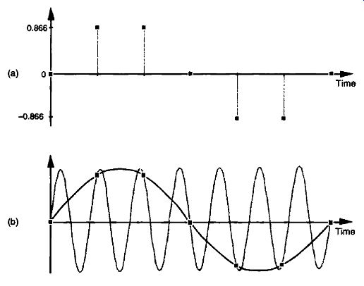
FIG. 1 Frequency ambiguity: (a) discrete-time sequence of values; (b) two different sinewaves that pass through the points of the discrete sequence.

1. ALIASING: SIGNAL AMBIGUITY IN THE FREQUENCY DOMAIN

There is a frequency-domain ambiguity associated with discrete-time signal samples that does not exist in the continuous signal world, and we can appreciate the effects of this uncertainty by understanding the sampled nature of discrete data. By way of example, suppose you were given the following sequence of values,

x(0) = 0 x(1) =0.866

x(2) -= 0.866

x(3) = 0

x(4)= -0.866

x(5)= -0.866

x(6)= 0,

and were told that they represent instantaneous values of a time-domain sinewave taken at periodic intervals. Next, you were asked to draw that sinewave.

You'd start by plotting the sequence of values shown by the dots in FIG. 1(a).

Next, you'd be likely to draw the sinewave, illustrated by the solid line in FIG. 1(b), that passes through the points representing the original sequence.

Another person, however, might draw the sinewave shown by the shaded ine in FIG. 1(b). We see that the original sequence of values could, with equal validity, represent sampled values of both sinewaves. The key issue is that, if the data sequence represented periodic samples of a sinewave, we cannot unambiguously determine the frequency of the sinewave from those sample values alone.

Reviewing the mathematical origin of this frequency ambiguity enables us not only to deal with it, but to use it to our advantage.

Let's derive an expression for this frequency-domain ambiguity and, then, look at a few specific examples. Consider the continuous time-domain sinusoidal signal defined as

x(t) = sin(2 pi f0 t) . (eqn. 1)

This x(t) signal is a garden variety sinewave whose frequency is f, Hz. Now let's sample x(t) at a rate off, samples/s, i.e., at regular periods of t, seconds where t, = 1/f,. If we start sampling at time t = 0, we will obtain samples at times Oi s, 1 t, 2„ and so on. So, from Eq. (eqn. 1), the first n successive samples have the values'

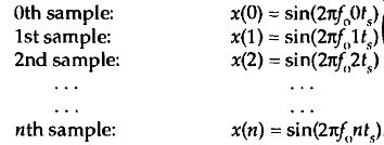
(eqn. 2)

Equation (eqn. 2) defines the value of the nth sample of our x(n) sequence to be equal to the original sinewave at the time instant nt,. Because two values of a sinewave are identical if they're separated by an integer multiple of 2E radians, i.e., sin(0) = sin(0+2nm) where m is any integer, we can modify Eq. (eqn. 2) as

(eqn. 3)

If we let m be an integer multiple of n, m = kn, we can replace the min ratio in Eq. (eqn. 3) with k so that

(eqn. 4)

Because f, = 1/1. , , we can equate the x(n) sequences in Eqs. (eqn. 2) and (eqn. 4) as x(n) = sin(2 pi f0 nt,) = sin(27t(fo+kf s )nts ) .

(eqn. 5)

The fo and (fo+kf,) factors in Eq. (eqn. 5) are therefore equal. The implication of Eq. (eqn. 5) is critical. It means that an x(n) sequence of digital sample values, representing a sinewave off, Hz, also exactly represents sinewaves at other frequencies, namely, f ) + kfs . This is one of the most important relationships in the field of digital signal processing. It's the thread with which all sampling schemes are woven. In words, Eq. (eqn. 5) states that

When sampling at a rate off, samples s, if k is any positive or negative integer, we cannot distinguish between the sampled values of a sinewave of f.

Hz and a sinewave of (fol-kfs) Hz. (eqn. 2)

x(n) = sin(2Ef0nt,).

It's true. No sequence of values stored in a computer, for example, can unambiguously represent one and only one sinusoid without additional in- formation. This fact applies equally to A /D-converter output samples as well as signal samples generated by computer software routines. The sampled nature of any sequence of discrete values makes that sequence also represent an infinite number of different sinusoids.

Equation (eqn. 5) influences all digital signal processing schemes. It's the reason that, although we've only shown it for sinewaves, we'll see in Section 3 that the spectrum of any discrete series of sampled values contains periodic replications of the original continuous spectrum. The period between these replicated spectra in the frequency domain will always be fs, and the spectral replications repeat all the way from DC to daylight in both directions of the frequency spectrum. That's because k in Eq. (eqn. 5) can be any positive or negative integer. (In Sections 5 and 6, we'll learn that Eq. (eqn. 5) is the reason that all digital filter frequency responses are periodic in the frequency domain and is crucial to analyzing and designing a popular type of digital filter known as the infinite impulse response filter.)

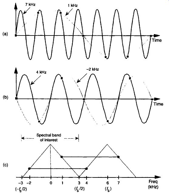
FIG. 2 Frequency ambiguity effects of Eq. (eqn. 5): (a) sampling a 7-kHz sinewave at a sample rate of 6 kHz: (b) sampling a 4-kHz sinewave at a sample rate of 6 kHz; (c) spectral relationships showing aliasing of the 7- and 4-kHz sinewaves.

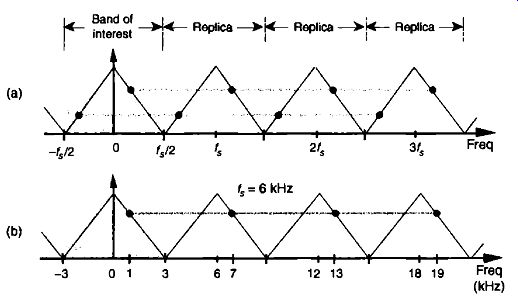
FIG. 3 Shark's tooth pattern: (a) aliasing at multiples of the sampling frequency; (b) aliasing of the 7-kHz sinewave to 1 kHz, 13 kHz, and 19 kHz.

To illustrate the effects of Eq. (eqn. 5), let's build on FIG. 1 and consider the sampling of a 7-kHz sinewave at a sample rate of 6 kHz. A new sample is determined every 1/6000 seconds, or once every 167 microseconds, and their values are shown as the dots in FIG. 2(a). Notice that the sample values would not change at all if, instead, we were sampling a 1-kHz sinewave. In this example fo = 7 kHz, fs. = 6 kHz, and k = -1 in Eq. (eqn. 5), such that fo-Fkfs.= [7+(-1.6)] = 1 kHz. Our problem is that no processing scheme can determine if the sequence of sampled values, whose amplitudes are represented by the dots, came from a 7-kHz or a 1-kHz sinusoid. If these amplitude values are applied to a digital process that detects energy at 1 kHz, the detector output would indicate energy at 1 kHz. But we know that there is no 1-kHz tone there-our input is a spectrally pure 7-kHz tone. Equation (eqn. 5) is causing a sinusoid, whose name is 7 kHz, to go by the alias of 1 kHz. Asking someone to determine which sinewave frequency ac counts for the sample values in FIG. 2(a) is like asking them "When I add two numbers I get a sum of four. What are the two numbers?" The answer is that there is an infinite number of number pairs that can add up to four.

FIG. 2(b) shows another example of frequency ambiguity, that we'll call aliasing, where a 4-kHz sinewave could be mistaken for a -2-kHz sinewave. In FIG. 2(b), fo = 4 kHz, f, = 6 kHz, and k = -1 in Eq. (eqn. 5), so that fo+kf s. = [4+(-1 6)] = -2 kHz. Again, if we examine a sequence of numbers representing the dots in FIG. 2(b), we could not determine if the sampled sinewave was a 4-kHz tone or a -2-kHz tone. (Although the concept of negative frequencies might seem a bit strange, it provides a beautifully consistent methodology for predicting the spectral effects of sampling. Section 8 discusses negative frequencies and how they relate to real and complex signals.) Now, if we restrict our spectral band of interest to the frequency range of ±4/2 Hz, the previous two examples take on a special significance. The frequency A/2 is an important quantity in sampling theory and is referred to by different names in the literature, such as critical Nyquist, half Nyquist, and folding frequency. A graphical depiction of our two frequency aliasing examples is provided in FIG. 2(c). We're interested in signal components that are aliased into the frequency band between -A/2 and +A/2. Notice in FIG. 2(c) that, within the spectral band of interest ' (±3 kHz, because A = 6 kHz), there is energy at -2 kHz and +1 kHz, aliased from 4 kHz and 7 kHz, respectively. Note also that the vertical positions of the dots in FIG. 2(c) have no amplitude significance but that their horizontal positions indicate which frequencies are related through aliasing.

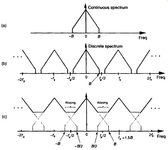
FIG. 4 Spectral replications: (a) original continuous signal spectrum; (b) spectral replications of the sampled signal when f5 /2 > (c) frequency overlap and aliasing when the sampling rate is too low because fs /2 < B.

A general illustration of aliasing is provided in the shark's tooth pattern in FIG. 3(a). Note how the peaks of the pattern are located at integer multiples of fs Hz. The pattern shows how signals residing at the intersection of a horizontal line and a sloped line will be aliased to all of the intersections of that horizontal line and all other lines with like slopes. For example, the pat tern in FIG. 3(h) shows that our sampling of a 7-kHz sinewave at a sample rate of 6 kHz will provide a discrete sequence of numbers whose spectrum ambiguously represents tones at 1 kHz, 7 kHz, 13 kHz, 19 kHz, etc.

Let's pause for a moment and let these very important concepts soak in a bit.

Again, discrete sequence representations of a continuous signal have unavoidable ambiguities in their frequency domains. These ambiguities must be taken into account in all practical digital signal processing algorithms.

OK, let's review the effects of sampling signals that are more interesting than just simple sinusoids.

2. SAMPLING LOW-PASS SIGNALS

Consider sampling a continuous real signal whose spectrum is shown in FIG. 4(a). Notice that the spectrum is symmetrical about zero Hz, and the spectral amplitude is zero above +13 Hz and below -B Hz, i.e., the signal is band-limited. (From a practical standpoint, the term band-limited signal merely implies that any signal energy outside the range of ±B Hz is below the sensitivity of our system.) Given that the signal is sampled at a rate off, samples/s, we can see the spectral replication effects of sampling in Figure 24(b), showing the original spectrum in addition to an infinite number of replications, whose period of replication is f, Hz. (Although we stated in Section 1.1 that frequency-domain representations of discrete-time sequences are themselves discrete, the replicated spectra in FIG. 4(b) are shown as continuous lines, instead of discrete dots, merely to keep the figure from looking too cluttered. We'll cover the full implications of discrete frequency spectra in Section 3.) Let's step back a moment and understand FIG. 4 for all it's worth.

FIG. 4(a) is the spectrum of a continuous signal, a signal that can only exist in one of two forms. Either it's a continuous signal that can be sampled, through A /D conversion, or it is merely an abstract concept such as a mathematical expression for a signal. It cannot be represented in a digital machine in its current band-limited form. Once the signal is represented by a sequence of discrete sample values, its spectrum takes the replicated form of FIG. 4(b).

The replicated spectra are not just figments of the mathematics; they exist and have a profound effect on subsequent digital signal processing." The replications may appear harmless, and it's natural to ask, "Why care about spectral replications? We're only interested in the frequency band within ±4/2." Well, if we perform a frequency translation operation or induce a change in sampling rate through decimation or interpolation, the spectral replications will shift up or down right in the middle of the frequency range of interest #;/ 2 and could cause problems. Let's see how we can control the locations of those spectral replications.

In practical A/D conversion schemes, fs is always greater than 2B to separate spectral replications at the folding frequencies of 412. This very important relationship offs 2B is known as the Nyquist criterion. To illustrate why the term folding frequency is used, let's lower our sampling frequency to fs= 1.5B Hz. The spectral result of this undersampling is illustrated in FIG. 4(c). The spectral replications are now overlapping the original baseband spectrum centered about zero Hz. Limiting our attention to the band 4/2 Hz, we see two very interesting effects. First, the lower edge and upper edge of the spectral replications centered at +4 and now lie in our band of interest. This situation is equivalent to the original spectrum folding to the left at +f5 /2 and folding to the right at -4/2. Portions of the spectral replications now combine with the original spectrum, and the result is aliasing errors. The discrete sampled values associated with the spectrum of FIG. 4(c) no longer truly represent the original input signal. The spectral information in the bands of -B to -B/2 and B/2 to B Hz has been corrupted. We show the amplitude of the aliased regions in FIG. 4(c) as dashed lines because we don't really know what the amplitudes will be if aliasing occurs.

The second effect illustrated by FIG. 4(c) is that the entire spectral content of the original continuous signal is now residing in the band of interest between -f5 /2 and +f6 /2. This key property was true in FIG. 4(b) and will always be true, regardless of the original signal or the sample rate. This effect is particularly important when we're digitizing (A /D converting) continuous signals. It warns us that any signal energy located above +B Hz and below -B Hz in the original continuous spectrum of FIG. 4(a) will always end up in the band of interest after sampling, regardless of the sample rate. For this reason, continuous (analog) low-pass filters are necessary in practice.

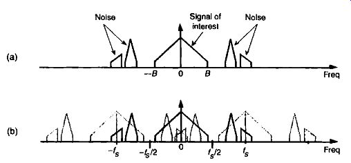
FIG. 5 Spectral replications: (a) original continuous signal plus noise spectrum; (b) discrete spectrum with noise contaminating the signal of interest.

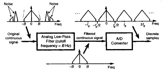
FIG. 6 Low-pass analog filtering prior to sampling at a rate of fs Hz.

We illustrate this notion by showing a continuous signal of bandwidth B accompanied by noise energy in FIG. 5(a). Sampling this composite continuous signal at a rate that's greater than 2B prevents replications of the signal of interest from overlapping each other, but all of the noise energy still ends up in the range between -A/2 and +A/2 of our discrete spectrum shown in FIG. 5(b). This problem is solved in practice by using an analog low pass anti-aliasing filter prior to A/D conversion to attenuate any unwanted signal energy above +B and below -B Hz as shown in FIG. 6. An example low-pass filter response shape is shown as the dotted line superimposed on the original continuous signal spectrum in FIG. 6. Notice how the output spectrum of the low-pass filter has been band-limited, and spectral aliasing is avoided at the output of the A/D converter.

This completes the discussion of simple low-pass sampling. Now let's go on to a more advanced sampling topic that's proven so useful in practice.

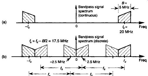
FIG. 7 Bandpass signal sampling: (a) original continuous signal spectrum; (b) sampled signal spectrum replications when sample rate is 17.5 MHz.

3. SAMPLING BANDPASS SIGNALS

Although satisfying the majority of sampling requirements, the sampling of low-pass signals, as in FIG. 6, is not the only sampling scheme used in practice. We can use a technique known as bandpass sampling to sample a continuous bandpass signal that is centered about some frequency other than zero Hz. When a continuous input signal's bandwidth and center frequency permit us to do so, bandpass sampling not only reduces the speed requirement of A/D converters below that necessary with traditional low-pass sampling; it also reduces the amount of digital memory necessary to capture a given time interval of a continuous signal.

By way of example, consider sampling the band-limited signal shown in FIG. 7(a) centered at fc = 20 MHz, with a bandwidth B = 5 MHz. We use the term bandpass sampling for the process of sampling continuous signals whose center frequencies have been translated up from zero Hz. What we're calling bandpass sampling goes by various other names in the literature, such as IF sampling, harmonic sampling [2], sub-Nyquist sampling, and under sampling (3). In bandpass sampling, we're more concerned with a signal's bandwidth than its highest frequency component. Note that the negative frequency portion of the signal, centered at -fc, is the mirror image of the positive frequency portion-as it must be for real signals. Our bandpass signal's highest frequency component is 22.5 MHz. Conforming to the Nyquist criterion (sampling at twice the highest frequency content of the signal) implies that the sampling frequency must be a minimum of 45 MHz. Consider the effect if the sample rate is 17.5 MHz shown in FIG. 7(b). Note that the original spectral components remain located at 2, and spectral replications are located exactly at baseband, i.e., butting up against each other at zero Hz. FIG. 7b) shows that sampling at 45 MHz was unnecessary to avoid aliasing--instead we've used the spectral replicating effects of Eq. (eqn. 5) to our advantage.

Bandpass sampling performs digitization and frequency translation in a single process, often called sampling translation. The processes of sampling and frequency translation are intimately bound together in the world of digital signal processing, and every sampling operation inherently results in spectral replications. The inquisitive reader may ask, "Can we sample at some still lower rate and avoid aliasing?" The answer is yes, but, to find out how, we have to grind through the derivation of an important bandpass sampling relationship. Our reward, however, will be worth the trouble because here's where bandpass sampling really gets interesting.

Let's assume we have a continuous input bandpass signal of bandwidth B. Its carrier frequency is fc Hz, i.e., the band pass signal is centered at fc Hz, and its sampled value spectrum is that shown in FIG. 8(a). We can sample that continuous signal at a rate, say f,, Hz, so the spectral replications of the positive and negative bands, Q and P, just butt up against each other exactly at zero Hz.

This situation, depicted in FIG. 8(a), is reminiscent of FIG. 7(b). With an arbitrary number of replications, say m, in the range of 2fc-B, we see that

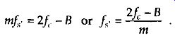
(eqn. 6)

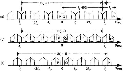
FIG. 8 Bandpass sampling frequency limits: (a) sample rate fs . (2fr - B)16; (b) sample rate Is less than fs .: (c) minimum sample rate fs’ < fs.

In FIG. 8(a), m 6 for illustrative purposes only. Of course nt can be any positive integer so long as f,, is never less than 2 13 . lithe sample rate L, is increased, the original spectra (bold) do not shift, but all the replications will shift. At zero Hz, the P band will shift to the right, and the Q band will shift to the left. These replications will overlap and aliasing occurs. Thus, from Eq. (eqn. 6), for an arbitrary in, there is a frequency that the sample rate must not exceed, or:

(eqn. 7)

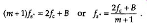
If we reduce the sample rate below the fe value shown in FIG. 8(a), the spacing between replications will decrease in the direction of the arrows in FIG. 8(b). Again, the original spectra do not shift when the sample rate is changed. At some new sample rate fs„, where fe, < f, the replication P' will just butt up against the positive original spectrum centered at fc as shown in FIG. 8(c). In this condition, we know that

(eqn. 8)

Should L„ be decreased in value, P' will shift further down in frequency and start to overlap with the positive original spectrum at L and aliasing occurs.

Therefore, from Eq. (eqn. 8) and for m+1, there is a frequency that the sample rate must always exceed, or +B m +1

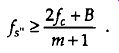
(eqn. 9)

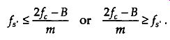
We can now combine Eqs. (eqn. 7) and (eqn. 9) to say that J . , may be chosen any where in the range between f,„ and 4, to avoid aliasing, or

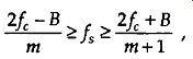
(eqn. 10)

where in is an arbitrary, positive integer ensuring that f, 2B. (For this type of periodic sampling of real signals, known as real or first-order sampling, the Nyquist critenonf5 a 2B must still be satisfied.)

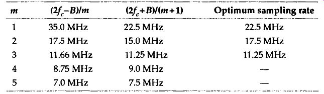
Table 1 Equation (eqn. 10) Applied to the Bandpass Signal Example

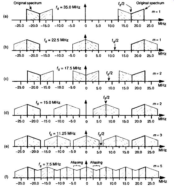
FIG. 9 Various spectral replications from Table 2-1: (a) fs = 35 MHz; (b) fs = 22.5 MHz; (c) fs = 17.5 MHz; (d) fs = 15 MHz; (e) f s = 11.25 MHz; (f) fs = 7.5 MHz.

To appreciate the important relationships in Eq. (eqn. 10), let's return to our bandpass signal example, where Eq. (eqn. 10) enables the generation of Table 2-1. This table tells us that our sample rate can be anywhere in the range of 22.5 to 35 MHz, anywhere in the range of 15 to 17.5 MHz, or any where in the range of 11.25 to 11.66 MHz. Any sample rate below 11.25 MHz is unacceptable because it will not satisfy Eq. (eqn. 10) as well as f, a 2B. The spectra resulting from several of the sampling rates from Table 1 are shown in FIG. 9 for our bandpass signal example. Notice in FIG. 9(f) that when'', equals 7.5 MHz (in = 5), we have aliasing problems because neither the greater than relationships in Eq. (eqn. 10) nor f,?. 2B have been satisfied. The m = 4 condition is also unacceptable because"- , 2B is not satisfied. The last column in Table 2-1 gives the optimum sampling frequency for each acceptable m value. Optimum sampling frequency is defined here as that frequency where spectral replications do not butt up against each other except at zero Hz. For example, in the m = 1 range of permissible sampling frequencies, it is much easier to perform subsequent digital filtering or other processing on the signal samples whose spectrum is that of FIG. 9(b), as opposed to the spectrum in FIG. 9(a). The reader may wonder, "Is the optimum sample rate always equal to the minimum permissible value for f, using Eq. (eqn. 10)?" The answer depends on the specific application-perhaps there are certain system constraints that must be considered. For example, in digital telephony, to simplify the follow on processing, sample frequencies are chosen to be integer multiples of 8 kHz[4]. Another application-specific factor in choosing the optimum f, is the shape of analog anti-aliasing filters[5]. Often, in practice, high-performance A/D converters have their hardware components fine-tuned during manufacture to ensure maximum linearity at high frequencies (>5 MHz). Their use at lower frequencies is not recommended.

An interesting way of illustrating the nature of Eq. (eqn. 10) is to plot the minimum sampling rate, (2L+B)/(m+1), for various values of m, as a function of R defined as

R = highest signal frequency component f, + B /2 bandwidth = B

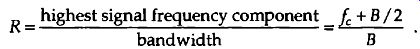
(eqn. 11)

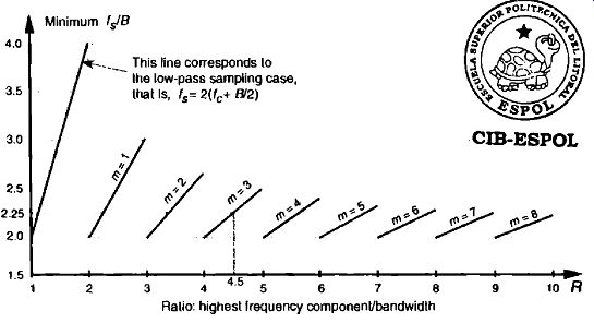
FIG. 10 Minimum bandpass sampling rate from Eq. (eqn. 10).

If we normalize the minimum sample rate from Eq. (eqn. 10) by dividing it by the bandwidth B, we get a bold-line plot whose axes are normalized to the bandwidth shown as the solid curve in FIG. 10. This figure shows us the minimum normalized sample rate as a function of the normalized highest frequency component in the bandpass signal. Notice that, regardless of the value of R, the minimum sampling rate need never exceed 4B and approaches 2B as the carrier frequency increases. Surprisingly, the minimum acceptable sampling frequency actually decreases as the bandpass signal's carrier frequency increases. We can interpret FIG. 10 by reconsidering our bandpass signal example from FIG. 7 where R = 22.5/5 = 4.5. This R value is indicated by the dashed line in FIG. 10 showing that m = 3 and fs / B is 2.25. With B = 5 MHz, then, the minimum f, = 11.25 MHz in agreement with Table 1. The leftmost line in FIG. 10 shows the low-pass sampling case, where the sample rate f, must be twice the signal's highest frequency component. So the normalized sample rate fs / B is twice the highest frequency component over B or 2R.

FIG. 10 has been prominent in the literature, but its normal presentation enables the reader to jump to the false conclusion that any sample rate above the minimum shown in the figure will be an acceptable sample rate. There's a clever way to avoid any misunderstanding [13]. If we plot the acceptable ranges of bandpass sample frequencies from Eq. (eqn. 10) as a function of R we get the depiction shown in FIG. 11. As we saw from Eq. (eqn. 10), Table 1, and FIG. 9, acceptable bandpass sample rates are a series of frequency ranges separated by unacceptable ranges of sample rate frequencies, that is, an acceptable bandpass sample frequency must be above the minimum shown in FIG. 10, but cannot be just any frequency above that minimum. The shaded region in FIG. 11 shows those normalized bandpass sample rates that will lead to spectral aliasing. Sample rates within the white regions of FIG. 11 are acceptable. So, for bandpass sampling, we want our sample rate to be in the white wedged areas associated with some value of In from Eq. (eqn. 10). Let's understand the significance of FIG. 11 by again using our previous bandpass signal example from FIG. 7.

FIG. 12 shows our bandpass signal example R value (highest frequency component/bandwidth) of 4.5 as the dashed vertical line. Because that line intersects just three white wedged areas, we see that there are only three frequency regions of acceptable sample rates, and this agrees with our results from Table 2-1. The intersection of the R = 4.5 line and the borders of the white wedged areas are those sample rate frequencies listed in Table 1.

So FIG. 11 gives a depiction of bandpass sampling restrictions much more realistic than that given in FIG. 10.

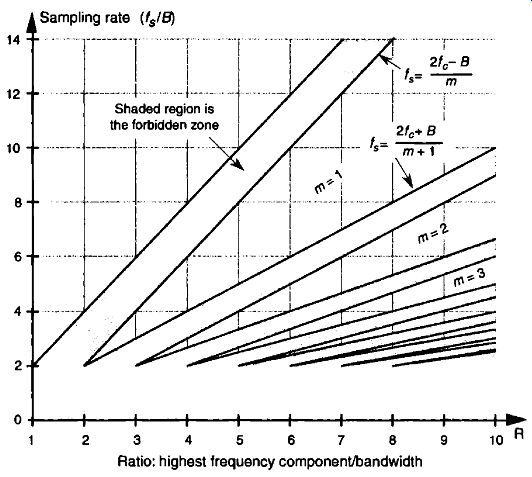
FIG. 11 Regions of acceptable bandpass sampling rates from Eq. (eqn. 10), normalized to the sample rate over the signal bandwidth (fs/B).

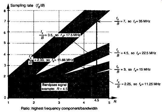
FIG. 12 Acceptable sample rates for the bandpass signal example (B = 5 MHz) with a value of R. 4.5.

Although Figures 11 and 12 indicate that we can use a sample rate that lies on the boundary between a white and shaded area, these sample rates should be avoided in practice. Nonideal analog bandpass filters, sample rate clock generator instabilities, and slight imperfections in available A/D converters make this ideal case impossible to achieve exactly. It's prudent to keep fs somewhat separated from the boundaries. Consider the bandpass sampling scenario shown in FIG. 13. With a typical (nonideal) analog bandpass filter, whose frequency response is indicated by the dashed line, it's prudent to consider the filter's bandwidth not as B, but as Bgb in our equations. That is, we create a guard band on either side of our filter so that there can be a small amount of aliasing in the discrete spectrum without distorting our desired signal, as shown at the bottom of FIG. 13.

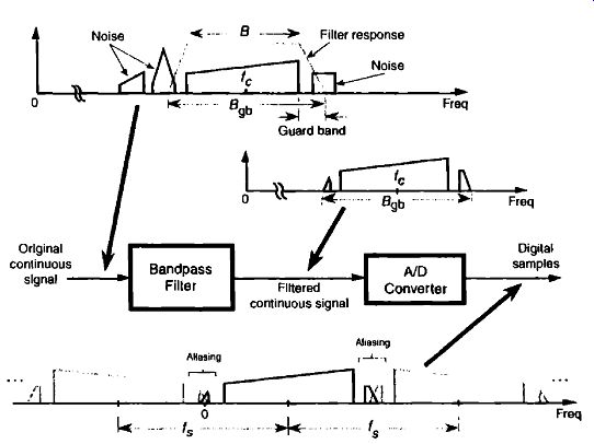
FIG. 13 Bandpass sampling with aliasing occurring only in the filter guard bands.

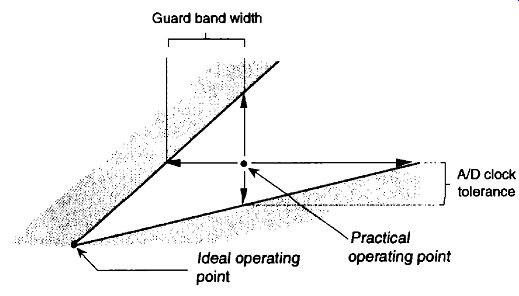
FIG. 14 Typical operating point for f s to compensate for nonideal hardware.

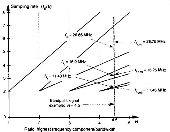
FIG. 15 Intermediate f_si and f_scntr operating points, from Eqs. (eqn. 12) and (eqn. 13), to avoid operating at the shaded boundaries for the band pass signal example. 13= 5 MHz and R= 4.5.

We can relate this idea of using guard bands to FIG. 11 by looking more closely at one of the white wedges. As shown in FIG. 14, we'd like to set our sample rate as far down toward the vertex of the white area as we can-lower in the wedge means a lower sampling rate. However, the closer we operate to the boundary of a shaded area, the more narrow the guard band must be, requiring a sharper analog bandpass filter, as well as the tighter the tolerance we must impose on the stability and accuracy of our A/D clock generator. (Remember, operating on the boundary between a white and shaded area in FIG. 11 causes spectral replications to butt up against each other.) So, to be safe, we operate at some intermediate point away from any shaded boundaries as shown in FIG. 14. Further analysis of how guard bandwidths and A/D clock parameters relate to the geometry of FIG. 14 is available in reference. For this discussion, we'll just state that it's a good idea to ensure that our selected sample rate does not lie too close to the boundary between a white and shaded area in FIG. 11.

There are a couple of ways to make sure we're not operating near a boundary. One way is to set the sample rate in the middle of a white wedge for a given value of R. We do this by taking the average between the maxi mum and minimum sample rate terms in Eq. (eqn. 10) for a particular value of m, that is, to center the sample rate operating point within a wedge we use a sample rate of

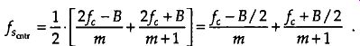
(eqn. 12)

Another way to avoid the boundaries of FIG. 14 is to use the following expression to determine an intermediate f. operating point:

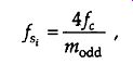
(eqn. 13)

where M_odd is an odd integer. Using Eq. (eqn. 13) yields the useful property that the sampled signal of interest will be centered at one fourth the sample rate (f,14). This situation is attractive because it greatly simplifies follow-on complex down-conversion (frequency translation) used in many digital communications applications. Of course the choice of M_odd must ensure that the Nyquist restriction of > 2B be satisfied. We show the results of Eqs. (eqn. 12) and (eqn. 13) for our bandpass signal example in FIG. 15.

4. SPECTRAL INVERSION IN BANDPASS SAMPLING

Some of the permissible f, values from Eq. (eqn. 10) will, although avoiding aliasing problems, provide a sampled baseband spectrum (located near zero Hz) that is inverted from the original positive and negative spectral shapes, that is, the positive baseband will have the inverted shape of the negative half from the original spectrum. This spectral inversion happens whenever m, in Eq. (eqn. 10), is an odd integer, as illustrated in Figures 9(b) and 9(e). When the original positive spectral bandpass components are symmetrical about the fc frequency, spectral inversion presents no problem and any non-aliasing value for f, from Eq. (eqn. 10) may be chosen. However, if spectral inversion is something to be avoided, for example, when single sideband signals are being processed, the minimum applicable sample rate to avoid spectral inversion is defined by Eq. (eqn. 10) with the restriction that m is the largest even integer such that f, 28 is satisfied. Using our definition of optimum sampling rate, the expression that provides the optimum noninverting sampling rates and avoids spectral replications butting up against each other, except at zero Hz, is

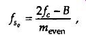
(eqn. 14)

where m even = 2, 4, 6, etc. For our bandpass signal example, Eq. (eqn. 14) and m = 2 provide an optimum noninverting sample rate of fso := 17.5 MHz, as shown in FIG. 9(c). In this case, notice that the spectrum translated toward zero Hz has the same orientation as the original spectrum centered at 20 MHz.

Then again, if spectral inversion is unimportant for your application, we can determine the absolute minimum sampling rate without having to choose various values for m in Eq. (eqn. 10) and creating a table like we did for Table 1. Considering FIG. 16, the question is "How many replications of the positive and negative images of bandwidth B can we squeeze into the frequency range of 2f, + B without overlap?" That number of replications is

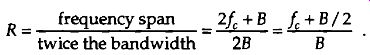
(eqn. 15)

To avoid overlap, we have to make sure that the number of replications is an integer less than or equal to R in Eq. (eqn. 15). So, we can define the integral number of replications to be Rint where

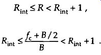
(eqn. 16)

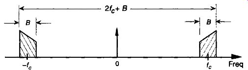
FIG. 16 Frequency span of a continuous bandpass signal.

With Rim replications in the frequency span of 2fc + B, then, the spectral repetition period, or minimum sample rate fs_min, is

(eqn. 17)

In our bandpass signal example, finding fs_min . first requires the appropriate value for R in Eq. (eqn. 16) as

[…]

so Rint = 4.

Then, from Eq. (eqn. 17), f 11 = (40+5)/4 = 11.25 MHz, which is the sample rate illustrated in Figures 9(e) and 12. So, we can use Eq. (eqn. 17) and avoid using various values for m in Eq. (eqn. 10) and having to create a table like Table 1. (Be careful though. Eq. (eqn. 17) places our sampling rate at the boundary between a white and shaded area of FIG. 12, and we have to consider the guard band strategy discussed above.) To recap the bandpass signal example, sampling at 11.25 MHz, from Eq. (eqn. 17), avoids aliasing and inverts the spectrum, while sampling at 17.5 MHz, from Eq. (eqn. 14), avoids aliasing with no spectral inversion.

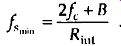
Now here's some good news. With a little additional digital processing, we can sample at 11.25 MHz, with its spectral inversion and easily re-invert the spectrum back to its original orientation. The discrete spectrum of any digital signal can be inverted by multiplying the signal's discrete-time samples by a sequence of alternating plus ones and minus ones (1, -1, 1, -1, etc.), indicated in the literature by the succinct expression (-1). This scheme allows bandpass sampling at the lower rate of Eq. (eqn. 17) while correcting for spectral inversion, thus avoiding the necessity of using the higher sample rates from Eq. (eqn. 14). Although multiplying time samples by (-1) is explored in detail in Section 13.1, all we need to remember at this point is the simple rule that multiplication of real signal samples by (-1)" is equivalent to multiplying by a co sine whose frequency is L/2. In the frequency domain, this multiplication flips the positive frequency band of interest, from zero to +4/2 Hz, about f,/4 Hz, and flips the negative frequency band of interest, from -f,/2 to zero Hz, about -4/4 Hz as shown in FIG. 17. The (-1) sequence is not only used for inverting the spectra of bandpass sampled sequences; it can be used to invert the spectra of low-pass sampled signals. 13e aware, however, that, in the low-pass sampling case, any DC (zero Hz) component in the original continuous signal will be translated to both +fs /2 and -4/2 after multiplication by (-1). In the literature of DSP, occasionally you'll see the (-1)" sequence represented by the equivalent expressions cos(pi n) and e1 ". We conclude this topic by consolidating in Table 2 what we need to know about bandpass sampling.

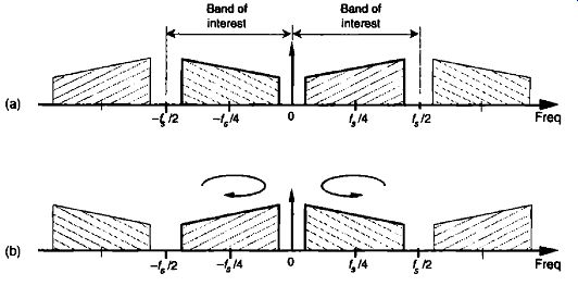
FIG. 17 Spectral inversion through multiplication by (-1)n: (a) original spectrum of a time-domain sequence; (b) new spectrum of the product of original time sequence and the (-1)" sequence.

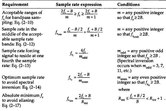
Table 2 Bandpass Sampling Relationships

REFERENCES

[1] Crochiere, R.E. and Rabiner, L.R. "Optimum FIR Digital Implementations for Decimation, Interpolation, and Narrow-band Filtering," IEEE Trans. on Acoust. Speech, and Signal Proc., Vol. ASSP-23, No. 5, October 1975.

[2] Steyskal, H. "Digital Beam forming Antennas," Microwave Journal, January 1987.

[3] Hill, G. "The Benefits of Undersampling," Electronic Design, July 11, 1994.

[4] Yam, E, and Redman, M. "Development of a 60-channel TDM-TDM Transmultiplexer," COMSAT Technical Review, Vol. 13, No. 1, Spring 1983.

[5] Floyd, P., and Taylor, J. "Dual-Channel Space Quadrature-Interferometer System," Microwave System Designer's Handbook, Fifth Edition, Microwave Systems News, 1987.

[6] Lyons, R. G. "How Fast Must You Sample," Test and Measurement World, November 1988.

[7] Stremler, F. Introduction to Communication Systems, Section 3, Second Edition, Addison Wesley Publishing Co., Reading, Massachusetts, p. 125.

[8] Webb, R. C. "IF Signal Sampling Improves Receiver Detection Accuracy," Microwaves & RF, March 1989.

[9] Haykin, S. Communications Systems, Section 7, John Wiley and Sons, New York, 1983, p. 376.

[10] Feldman, C. B., and Bennett, W. R. "Bandwidth and Transmission Performance," Bell System Tech. Journal, Vol. 28, 1989, p. 490.

[11] Panter, P. F. Modulation Noise, and Spectral Analysis, McGraw, New York, 1965, p. 527.

[12] Shanmugam, K. S. Digital and Analogue Communications Systems, John Wiley and Sons, New York, 1979, p. 378.

[13] Vaughan, R., Scott, N. and White, D. "The Theory of Bandpass Sampling," IEEE Trans. on Signal Processing, Vol. 39, No. 9, September 1991, pp. 1973-1984.

[14] Xenakis B., and Evans, A. "Vehicle Locator Uses Spread Spectrum Technology," RV De sign, October 1992.

PREV. | NEXT

Related Articles -- Top of Page -- Home