Digital Audio Compression [part 2]

<< cont. from part 1

10. Transform coding

Many transform coders use the discrete cosine transform described in section 3.31. The DCT works on blocks of samples which are windowed.

For simplicity the following example uses a very small block of only eight samples whereas a real encoder might use several hundred.

FIG. 18 shows the table of basis functions or wave table for an eight point DCT. Adding these two-dimensional waveforms together in different proportions will give any combination of the original eight PCM audio samples. The coefficients of the DCT simply control the proportion of each wave which is added in the inverse transform. The top-left wave has no modulation at all because it conveys the DC component of the block. Increasing the DC coefficient adds a constant amount to every sample in the block.

Moving to the right the coefficients represent increasing frequencies.

All these coefficients are bipolar, where the polarity indicates whether the original waveform at that frequency was inverted.

FIG. 19 shows an example of an inverse transform. The DC coefficient produces a constant level throughout the sample block. The remaining waves in the table are AC coefficients. A zero coefficient would result in no modulation, leaving the DC level unchanged. The wave next to the DC component represents the lowest frequency in the transform which is half a cycle per block. A positive coefficient would increase the signal voltage at the left side of the block whilst reducing it on the right, whereas a negative coefficient would do the opposite. The magnitude of the coefficient determines the amplitude of the wave which is added.

FIG. 19 also shows that the next wave has a frequency of one cycle per block, i.e. the waveform is made more positive at both sides and more negative in the middle.

Consequently an inverse DCT is no more than a process of mixing various waveforms from the wave table where the relative amplitudes and polarity of these patterns are controlled by the coefficients. The original transform is simply a mechanism which finds the coefficient amplitudes from the original PCM sample block.

The DCT itself achieves no compression at all. The number of coefficients which are output always equals the number of audio samples in the block. However, in typical program material, not all coefficients will have significant values; there will often be a few dominant coefficients. The coefficients representing the higher frequencies will often be zero or of small value, due to the typical energy distribution of audio.

Coding gain (the technical term for reduction in the number of bits needed) is achieved by transmitting the low-valued coefficients with shorter wordlengths. The zero-valued coefficients need not be transmitted at all. Thus it is not the DCT which compresses the audio, it is the subsequent processing. The DCT simply expresses the audio samples in a form which makes the subsequent processing easier.

Higher compression factors require the coefficient wordlength to be further reduced using requantizing. Coefficients are divided by some factor which increases the size of the quantizing step. The smaller number of steps which results permits coding with fewer bits, but of course with an increased quantizing error. The coefficients will be multiplied by a reciprocal factor in the decoder to return to the correct magnitude.

Further redundancy in transform coefficients can also be identified.

This can be done in various ways. Within a transform block, the coefficients may be transmitted using differential coding so that the first coefficient is sent in an absolute form whereas the remainder are transmitted as differences with respect to the previous one. Some coders attempt to predict the value of a given coefficient using the value of the same coefficient in typically the two previous blocks. The prediction is subtracted from the actual value to produce a prediction error or residual which is transmitted to the decoder. Another possibility is to use prediction within the transform block. The predictor scans the coefficients from, say, the low-frequency end upwards and tries to predict the value of the next coefficient in the scan from the values of the earlier coefficients. Again a residual is transmitted.

Inter-block prediction works well for stationary material, whereas intra-block prediction works well for transient material. An intelligent coder may select a prediction technique using the input entropy in the same way that it selects the window size.

Inverse transforming a requantized coefficient means that the frequency it represents is reproduced in the output with the wrong amplitude. The difference between the original and the reconstructed amplitude is considered to be a noise added to the wanted data. The audibility of such noise depends on the degree of masking prevailing.

11. Compression formats

There are numerous formats intended for audio compression and these can be divided into international standards and proprietary designs.

The ISO (International Standards Organization) and the IEC (Inter national Electrotechnical Commission) recognized that compression would have an important part to play and in 1988 established the ISO/ IEC/MPEG (Moving Picture Experts Group) to compare and assess various coding schemes in order to arrive at an international standard for compressing video. The terms of reference were extended the same year to include audio and the MPEG/Audio group was formed.

MPEG audio coding is used for DAB (digital audio broadcasting) and for the audio content of digital television broadcasts to the DVB standard.

In the USA, it has been proposed to use an alternative compression technique for the audio content of ATSC (advanced television systems committee) digital television broadcasts. This is the AC-319 system developed by Dolby Laboratories. The MPEG transport stream structure has also been standardized to allow it to carry AC-3 coded audio. The digital video disk (DVD) can also carry AC-3 or MPEG audio coding.

Other popular proprietary codes include apt-X which is a mild compression factor/short delay codec and ATRAC which is the codec used in MiniDisc.

12. MPEG Audio compression

The subject of audio compression was well advanced when the MPEG/Audio group was formed. As a result it was not necessary for the group to produce ab initio codecs because existing work was considered suitable.

As part of the Eureka 147 project, a system known as MUSICAM [20] (Masking pattern adapted Universal Sub-band Integrated Coding And Multiplexing) was developed jointly by CCETT in France, IRT in Germany and Philips in the Netherlands. MUSICAM was designed to be suitable for DAB (digital audio broadcasting).

As a parallel development, the ASPEC [21] (Adaptive Spectral Perceptual Entropy Coding) system was developed from a number of earlier systems as a joint proposal by AT&T Bell Labs, Thomson, the Fraunhofer Society and CNET. ASPEC was designed for use at high compression factors to allow audio transmission on ISDN.

These two systems were both fully implemented by July 1990 when comprehensive subjective testing took place at the Swedish Broadcasting Corporation. [4,22,23]

As a result of these tests, the MPEG/Audio group combined the attributes of both ASPEC and MUSICAM into a standard [1,24] having three levels of complexity and performance.

These three different levels, which are known as layers, are needed because of the number of possible applications. Audio coders can be operated at various compression factors with different quality expectations. Stereophonic classical music requires different quality criteria from monophonic speech. The complexity of the coder will be reduced with a smaller compression factor. For moderate compression, a simple codec will be more cost effective. On the other hand, as the compression factor is increased, it will be necessary to employ a more complex coder to maintain quality.

MPEG Layer 1 is a simplified version of MUSICAM which is appropriate for the mild compression applications at low cost. Layer II is identical to MUSICAM and is used for DAB and for the audio content of DVB digital television broadcasts. Layer III is a combination of the best features of ASPEC and MUSICAM and is mainly applicable to telecommunications where high compression factors are required.

The approach of the ISO to standardization in MPEG Audio is novel because the encoder is not completely specified. FIG. 20(a) shows that instead the way in which a decoder shall interpret the bitstream is defined. A decoder which can successfully interpret the bitstream is said to be compliant. FIG. 20(b) shows that the advantage of standardizing the decoder is that over time encoding algorithms, particularly masking models, can improve yet compliant decoders will continue to function with them.

Manufacturers can supply encoders using algorithms which are proprietary and their details do not need to be published. A useful result is that there can be competition between different encoder designs which means that better designs will evolve. The user will have greater choice because different levels of cost and complexity can exist in a range of coders yet a compliant decoder will operate with them all.

MPEG is, however, much more than a compression scheme as it also standardizes the protocol and syntax under which it is possible to combine or multiplex audio data with video data to produce a digital equivalent of a television program. Many such programs can be combined in a single multiplex and MPEG defines the way in which such multiplexes can be created and transported. The definitions include the metadata which decoders require to de-multiplex correctly and which users will need to locate programs of interest.

At each layer, MPEG Audio coding allows input sampling rates of 32, 44.1 and 48 kHz and supports output bit rates of 32, 48, 56, 64, 96, 112, 128, 192, 256 and 384 kbits/s. The transmission can be mono, dual-channel (e.g. bilingual), or stereo. Another possibility is the use of joint stereo mode in which the audio becomes mono above a certain frequency. This allows a lower bit rate with the obvious penalty of reduced stereo fidelity.

The layers of MPEG Audio coding (I, II and III) should not be confused with the MPEG-1 and MPEG-2 television coding standards. MPEG-1 and MPEG-2 flexibly define a range of systems for video and audio coding, whereas the layers define types of audio coding.

FIG. 20 (a) MPEG defines the protocol of the bitstream between encoder and decoder. The decoder is defined by implication, the encoder is left very much to the designer. (b) This approach allows future encoders of better performance to remain compatible with existing decoders. (c) This approach also allows an encoder to produce a standard bitstream while its technical operation remains a commercial secret.

The earlier MPEG-1 standard compresses audio and video into about 1.5Mbits/s. The audio coding of MPEG-1 may be used on its own to encode one or two channels at bit rates up to 448 kbits/s. MPEG-2 allows the number of channels to increase to five: Left, Right, Centre, Left surround, Right surround and Subwoofer. In order to retain reverse compatibility with MPEG-1, the MPEG-2 coding converts the five channel input to a compatible two-channel signal, Lo,Ro, by matrixing25 as shown in FIG. 21. The data from these two channels are encoded in a standard MPEG-1 audio frame, and this is followed in MPEG-2 by an ancillary data frame which an MPEG-1 decoder will ignore. The ancillary frame contains data for another three audio channels. FIG. 22 shows that there are eight modes in which these three channels can be obtained.

The encoder will select the mode which gives the least data rate for the prevailing distribution of energy in the input channels. An MPEG-2 decoder will extract those three channels in addition to the MPEG-1 frame and then recover all five original channels by an inverse matrix which is steered by mode select bits in the bitstream.

The requirement for MPEG-2 Audio to be backward compatible with MPEG-1 audio coding was essential for some markets, but did com promise the performance because certain useful coding tools could not be used. Consequently the MPEG Audio group evolved a multi-channel standard which was not backward compatible because it incorporated additional coding tools in order to achieve higher performance. This came to be known as MPEG-2 AAC (advanced audio coding).

FIG. 21 To allow compatibility with two-channel systems, a stereo signal pair is derived from the five surround signals in this manner.

FIG. 22 In addition to sending the stereo compatible pair, one of the above combinations of signals can be sent. In all cases a suitable inverse matrix can recover the original five channels.

13. MPEG Layer I

FIG. 23 A simple sub-band coder. The bit allocation may come from analysis of FIG. 23 shows a block diagram of a Layer I coder which is a simplified version of that used in the MUSICAM system. A polyphase filter divides the audio spectrum into 32 equal sub-bands. The output of the filter bank is critically sampled. In other words the output data rate is no higher than the input rate because each band has been heterodyned to a frequency range from zero upwards.

Sub-band compression takes advantage of the fact that real sounds do not have uniform spectral energy. The wordlength of PCM audio is based on the dynamic range required and this is generally constant with frequency although any pre-emphasis will affect the situation. When a signal with an uneven spectrum is conveyed by PCM, the whole dynamic range is occupied only by the loudest spectral component, and all the other components are coded with excessive headroom. In its simplest form, sub-band coding works by splitting the audio signal into a number of frequency bands and companding each band according to its own level. Bands in which there is little energy result in small amplitudes which can be transmitted with short wordlength. Thus each band results in variable-length samples, but the sum of all the sample wordlengths is less than that of the PCM input and so a degree of coding gain can be obtained.

A Layer I-compliant encoder, i.e. one whose output can be understood by a standard decoder, can be made which does no more than this.

Provided the syntax of the bitstream is correct, the decoder is not concerned with how the coding decisions were made. However, higher compression factors require the distortion level to be increased and this should only be done if it is known that the distortion products will be masked. Ideally the sub-bands should be narrower than the critical bands of the ear. FIG. 14 showed the critical condition where the masking tone is at the top edge of the sub-band. The use of an excessive number of sub-bands will, however, raise complexity and the coding delay. The use of 32 equal sub-bands in MPEG Layers I and II is a compromise.

Efficient polyphase band-splitting filters can only operate with equal width sub-bands and the result, in an octave-based hearing model, is that sub-bands are too wide at low frequencies and too narrow at high frequencies.

To offset the lack of accuracy in the sub-band filter a parallel fast Fourier transform is used to drive the masking model. The standard suggests masking models, but compliant bitstreams can result from other models. In Layer I a 512-point FFT is used. The output of the FFT is used to determine the masking threshold which is the sum of all masking sources. Masking sources include at least the threshold of hearing which may locally be raised by the frequency content of the input audio. The degree to which the threshold is raised depends on whether the input audio is sinusoidal or atonal (broadband, or noise-like).

In the case of a sine wave, the magnitude and phase of the FFT at each frequency will be similar from one window to the next, whereas if the sound is atonal the magnitude and phase information will be chaotic.

The masking threshold is effectively a graph of just noticeable noise as a function of frequency. FIG. 24(a) shows an example. The masking threshold is calculated by convolving the FFT spectrum with the cochlea spreading function (see section 2.11) with corrections for tonality. The level of the masking threshold cannot fall below the absolute masking threshold which is the threshold of hearing.

The masking threshold is then superimposed on the actual frequencies of each sub-band so that the allowable level of distortion in each can be established. This is shown in FIG. 24(b).

Constant-size input blocks are used, containing 384 samples. At 48 kHz, 384 samples corresponds to a period of 8ms. After the sub-band filter each band contains 12 samples per block. The block size is too long to avoid the pre-masking phenomenon of FIG. 11. Consequently the masking model must ensure that heavy requantizing is not used in a block which contains a large transient following a period of quiet. This can be done by comparing parameters of the current block with those of the previous block as a significant difference will indicate transient activity.

The samples in each sub-band block or bin are companded according to the peak value in the bin. A six-bit scale factor is used for each sub-band which applies to all 12 samples. The gain step is 2 dB and so with a six-bit code over 120 dB of dynamic range is available.

A fixed-output bit rate is employed, and as there is no buffering the size of the coded output block will be fixed. The wordlengths in each bin will have to be such that the sum of the bits from all the sub-bands equals the size of the coded block. Thus some sub-bands can have long wordlength coding if others have short wordlength coding. The process of determining the requantization step size, and hence the wordlength in each sub-band, is known as bit allocation. In Layer I all sub-bands are treated in the same way and fourteen different requantization classes are used. Each one has an odd number of quantizing intervals so that all codes are referenced to a precise zero level.

FIG. 24 A continuous curve (a) of the just-noticeable noise level is calculated by the masking model. The levels of noise in each sub-band (b) must be set so as not to exceed the level of the curve.

Where masking takes place, the signal is quantized more coarsely until the distortion level is raised to just below the masking level. The coarse quantization requires shorter wordlengths and allows a coding gain. The bit allocation may be iterative as adjustments are made to obtain an equal NMR across all sub-bands. If the allowable data rate is adequate, a positive NMR will result and the decoded quality will be optimal.

However, at lower bit rates and in the absence of buffering a temporary increase in bit rate is not possible. The coding distortion cannot be masked and the best the encoder can do is to make the (negative) NMR equal across the spectrum so that artifacts are not emphasized unduly in any one sub-band. It is possible that in some sub-bands there will be no data at all, either because such frequencies were absent in the program material or because the encoder has discarded them to meet a low bit rate.

The samples of differing wordlength in each bin are then assembled into the output coded block. Unlike a PCM block, which contains samples of fixed wordlength, a coded block contains many different wordlengths which may vary from one sub-band to the next. In order to deserialize the block into samples of various wordlengths and de-multiplex the samples into the appropriate frequency bins, the decoder has to be told what bit allocations were used when it was packed, and some synchronizing means is needed to allow the beginning of the block to be identified.

The compression factor is determined by the bit-allocation system. It is trivial to change the output block size parameter to obtain a different compression factor. If a larger block is specified, the bit allocator simply iterates until the new block size is filled. Similarly the decoder need only deserialize the larger block correctly into coded samples and then the expansion process is identical except for the fact that expanded words contain less noise. Thus codecs with varying degrees of compression are available which can perform different bandwidth/performance tasks with the same hardware.

FIG. 25 (a) The MPEG Layer I data frame has a simple structure, (b) in the Layer II frame, the compression of the scale factors requires the additional SCFSI code described in the text.

FIG. 25(a) shows the format of the Layer I elementary stream. The frame begins with a sync pattern to reset the phase of deserialization, and a header which describes the sampling rate and any use of pre-emphasis.

Following this is a block of 32 four-bit allocation codes. These specify the wordlength used in each sub-band and allow the decoder to deserialize the sub-band sample block. This is followed by a block of 32 six-bit scale factor indices, which specify the gain given to each band during companding. The last block contains 32 sets of 12 samples. These samples vary in wordlength from one block to the next, and can be from 0 to 15 bits long. The de-serializer has to use the 32 allocation information codes to work out how to deserialize the sample block into individual samples of variable length.

The Layer I MPEG decoder is shown in FIG. 26. The elementary stream is deserialized using the sync pattern and the variable-length samples are assembled using the allocation codes. The variable-length samples are returned to fifteen-bit wordlength by adding zeros. The scale factor indices are then used to determine multiplication factors used to return the waveform in each sub-band to its original amplitude. The 32 sub-band signals are then merged into one spectrum by the synthesis filter. This is a set of bandpass filters which heterodynes every sub-band to the correct place in the audio spectrum and then adds them to produce the audio output.

FIG. 26 The Layer I decoder. See text for details.

14. MPEG Layer II

MPEG Layer II audio coding is identical to MUSICAM. The same 32-band filter bank and the same block companding scheme as Layer I is used. In order to give the masking model better spectral resolution, the side-chain FFT has 1024 points. The FFT drives the masking model which may be the same as is suggested for Layer I. The block length is increased to 1152 samples. This is three times the block length of Layer I, corresponding to 24ms at 48 kHz.

FIG. 25(b) shows the Layer II elementary stream structure.

Following the sync pattern the bit-allocation data are sent. The requantizing process of Layer II is more complex than in Layer I. The sub-bands are categorized into three frequency ranges, low, medium and high, and the requantizing in each range is different. Low-frequency samples can be quantized into 15 different wordlengths, mid-frequencies into seven different wordlengths and high frequencies into only three different wordlengths. Accordingly the bit-allocation data use words of four, three and two bits depending on the sub-band concerned. This reduces the amount of allocation data to be sent. In each case one extra combination exists in the allocation code. This is used to indicate that no data are being sent for that sub-band.

The 1152-sample block of Layer II is divided into three blocks of 384 samples so that the same companding structure as Layer I can be used. The 2 dB step size in the scale factors is retained. However, not all the scale factors are transmitted, because they contain a degree of redundancy. In real program material, the difference between scale factors in successive blocks in the same band exceeds 2 dB less than 10 per cent of the time. Layer II coders analyze the set of three successive scale factors in each sub-band.

On stationary program, these will be the same and only one scale factor out of three is sent. As the transient content increases in a given sub-band, two or three scale factors will be sent. A two-bit code known as SCFSI (scale factor select information) must be sent to allow the decoder to determine which of the three possible scale factors have been sent for each sub-band.

This technique effectively halves the scale factor bit rate.

As for Layer I, the requantizing process always uses an odd number of steps to allow a true centre zero step. In long wordlength codes this is not a problem, but when three, five or nine quantizing intervals are used, binary is inefficient because some combinations are not used. For example, five intervals needs a three-bit code having eight combinations leaving three unused.

The solution is that when three,-five-or nine-level coding is used in a sub-band, sets of three samples are encoded into a granule. FIG. 27 shows how granules work. Continuing the example of five quantizing intervals, each sample could have five different values, therefore all combinations of three samples could have 125 different values. As 128 values can be sent with a seven-bit code, it will be seen that this is more efficient than coding the samples separately as three five-level codes would need nine bits. The three requantized samples are used to address a look-up table which outputs the granule code. The decoder can establish that granule coding has been used by examining the bit-allocation data.

The requantized samples/granules in each sub-band, bit allocation data, scale factors and scale factor select codes are multiplexed into the output bitstream.

FIG. 27 Codes having ranges smaller than a power of two are inefficient. Here three codes with a range of five values which would ordinarily need 3 x 3 bits can be carried in a single eight-bit word.

FIG. 28 A Layer II decoder is slightly more complex than the Layer I decoder because of the need to decode granules and scale factors.

The Layer II decoder is shown in FIG. 28. This is not much more complex than the Layer I decoder. The demultiplexing will separate the sample data from the side information. The bit-allocation data will specify the wordlength or granule size used so that the sample block can be deserialized and the granules decoded. The scale factor select information will be used to decode the compressed scale factors to produce one scale factor per block of 384 samples. Inverse quantizing and inverse sub-band filtering takes place as for Layer I.

15. MPEG Layer III

Layer III is the most complex layer, and is only really necessary when the most severe data rate constraints must be met. It is also known as MP3 in its application of music delivery over the Internet. It is a transform code based on the ASPEC system with certain modifications to give a degree of commonality with Layer II. The original ASPEC coder used a direct MDCT on the input samples. In Layer III this was modified to use a hybrid transform incorporating the existing polyphase 32-band QMF of Layers I and II and retaining the block size of 1152 samples. In Layer III, the 32 sub-bands from the QMF are further processed by a critically sampled MDCT.

The windows overlap by two to one. Two window sizes are used to reduce pre-echo on transients. The long window works with 36 sub-band samples corresponding to 24ms at 48 kHz and resolves 18 different frequencies, making 576 frequencies altogether. Coding products are spread over this period which is acceptable in stationary material but not in the vicinity of transients. In this case the window length is reduced to 8ms. Twelve sub-band samples are resolved into six different frequencies making a total of 192 frequencies. This is the Heisenberg inequality: by increasing the time resolution by a factor of three, the frequency resolution has fallen by the same factor.

FIG. 29 The window functions of Layer III coding. At (a) is the normal long window, whereas (b) shows the short window used to handle transients. Switching between window sizes requires transition windows (c) and (d). An example of switching using transition windows is shown in (e).

FIG. 29 shows the available window types. In addition to the long and short symmetrical windows there is a pair of transition windows, know as start and stop windows which allow a smooth transition between the two window sizes. In order to use critical sampling, MDCTs must resolve into a set of frequencies which is a multiple of four. Switching between 576 and 192 frequencies allows this criterion to be met. Note that an 8ms window is still too long to eliminate pre-echo. Pre-echo is eliminated using buffering. The use of a short window minimizes the size of the buffer needed.

Layer III provides a suggested (but not compulsory) pycho-acoustic model which is more complex than that suggested for Layers I and II, primarily because of the need for window switching. Pre-echo is associated with the entropy in the audio rising above the average value and this can be used to switch the window size. The perceptive model is used to take advantage of the high-frequency resolution available from the DCT which allows the noise floor to be shaped much more accurately than with the 32 sub-bands of Layers I and II. Although the MDCT has high-frequency resolution, it does not carry the phase of the waveform in an identifiable form and so is not useful for discriminating between tonal and atonal inputs. As a result a side FFT which gives conventional amplitude and phase data is still required to drive the masking model.

Non-uniform quantizing is used, in which the quantizing step size becomes larger as the magnitude of the coefficient increases. The quantized coefficients are then subject to Huffman coding. This is a technique where the most common code values are allocated the shortest wordlength. Layer III also has a certain amount of buffer memory so that pre-echo can be avoided during entropy peaks despite a constant output bit rate.

FIG. 30 shows a Layer III encoder. The output from the sub-band filter is 32 continuous band-limited sample streams. These are subject to 32 parallel MDCTs. The window size can be switched individually in each sub-band as required by the characteristics of the input audio. The parallel FFT drives the masking model which decides on window sizes as well as producing the masking threshold for the coefficient quantizer. The distortion control loop iterates until the available output data capacity is reached with the most uniform NMR.

FIG. 30 The Layer III coder. Note the connection between the buffer and the quantizer which allows different frames to contain different amounts of data.

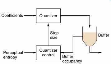
FIG. 31 The variable rate coding of Layer III. An approaching transient via the perceptual entropy signal causes the coder to quantize more heavily in order to empty the buffer. When the transient arrives, the quantizing can be made more accurate and the increased data can be accepted by the buffer.

The available output capacity can vary owing to the presence of the buffer. FIG. 31 shows that the buffer occupancy is fed back to the quantizer. During stationary program material, the buffer contents are deliberately run down by slight coarsening of the quantizing. The buffer empties because the output rate is fixed but the input rate has been reduced. When a transient arrives, the large coefficients which result can be handled by filling the buffer, avoiding raising the output bit rate whilst also avoiding the pre-echo which would result if the coefficients were heavily quantized.

FIG. 32 In Layer III, the logical frame rate is constant and is transmitted by equally spaced sync patterns. The data blocks do not need to coincide with sync. A pointer after each sync pattern specifies where the data block starts. In this example block 2 is smaller whereas 1 and 3 have enlarged.

In order to maintain synchronism between encoder and decoder in the presence of buffering, headers and side information are sent synchronously at frame rate. However, the position of boundaries between the main data blocks which carry the coefficients can vary with respect to the position of the headers in order to allow a variable frame size. FIG. 32 shows that the frame begins with an unique sync pattern which is followed by the side information. The side information contains a parameter called main data begin which specifies where the main data for the present frame began in the transmission. This parameter allows the decoder to find the coefficient block in the decoder buffer. As the frame headers are at fixed locations, the main data blocks may be interrupted by the headers.

16. MPEG-2 AAC

The MPEG standards system subsequently developed an enhanced system known as advanced audio coding (AAC). [8, 26]

This was intended to be a standard which delivered the highest possible performance using newly developed tools that could not be used in any standard which was backward compatible. AAC will also form the core of the audio coding of MPEG-4.

AAC supports up to 48 audio channels with default support of monophonic, stereo and 5.1 channel (3/2) audio. The AAC concept is based on a number of coding tools known as modules which can be combined in different ways to produce bitstreams at three different profiles.

The main profile requires the most complex encoder which makes use of all the coding tools. The low-complexity (LC) profile omits certain tools and restricts the power of others to reduce processing and memory requirements. The remaining tools in LC profile coding are identical to those in main profile such that a main profile decoder can decode LC profile bitstreams.

The scalable sampling rate (SSR) profile splits the input audio into four equal frequency bands each of which results in a self-contained bitstream. A simple decoder can decode only one, two or three of these bitstreams to produce a reduced bandwidth output. Not all the AAC tools are available to SSR profile.

The increased complexity of AAC allows the introduction of lossless coding tools. These allow a lower bit rate for the same quality or improved quality at a given bit rate where the reliance on lossy coding is reduced. There is greater attention given to the interplay between time-domain and frequency-domain precision in the human hearing system.

FIG. 33 shows a block diagram of an AAC main profile encoder.

The audio signal path is straight through the centre. The formatter assembles any side-chain data along with the coded audio data to produce a compliant bitstream. The input signal passes to the filter bank and the perceptual model in parallel.

FIG. 33 The AAC encoder. Signal flow is from left to right whereas side-chain data flow is vertical.

FIG. 34 In AAC short blocks must be used in multiples of 8 so that the long block phase is undisturbed. This keeps block synchronism in multichannel systems.

The filter bank consists of a 50 per cent overlapped critically sampled MDCT which can be switched between block lengths of 2048 and 256 samples. At 48 kHz the filter allows resolutions of 23Hz and 21ms or 187Hz and 2.6ms. As AAC is a multichannel coding system, block length switching cannot be done indiscriminately as this would result in loss of block phase between channels. Consequently if short blocks are selected, the coder will remain in short block mode for integer multiples of eight blocks. This is illustrated in FIG. 34 which also shows the use of transition windows between the block sizes as was done in Layer III.

The shape of the window function interferes with the frequency selectivity of the MDCT. In AAC it is possible to select either a sine window or a Kaiser-Bessel-derived (KBD) window as a function of the input audio spectrum. As was seen in section 3, filter windows allow different compromises between bandwidth and rate of roll-off. The KBD window rolls off later but is steeper and thus gives better rejection of frequencies more than about 200Hz apart whereas the sine window rolls off earlier but less steeply and so gives better rejection of frequencies less than 70Hz.

Following the filter bank is the intra-block predictive coding module.

When enabled this module finds redundancy between the coefficients within one transform block. In section 3 the concept of transform duality was introduced, in which a certain characteristic in the frequency domain would be accompanied by a dual characteristic in the time domain and vice versa. FIG. 35 shows that in the time domain, predictive coding works well on stationary signals but fails on transients. The dual of this characteristic is that in the frequency domain, predictive coding works well on transients but fails on stationary signals.

Equally, a predictive coder working in the time domain produces an error spectrum which is related to the input spectrum. The dual of this characteristic is that a predictive coder working in the frequency domain produces a prediction error which is related to the input time-domain signal.

FIG. 35 Transform duality suggests that predictability will also have a dual characteristic. A time predictor will not anticipate the transient in (a), whereas the broad spectrum of signal (a), shown in (b), will be easy for a predictor advancing down the frequency axis. In contrast, the stationary signal (c) is easy for a time predictor, whereas in the spectrum of (c) shown at (d) the spectral spike will not be predicted.

This explains the use of the term temporal noise shaping (TNS) used in the AAC documents. [27] When used during transients, the TNS module produces a distortion which is time-aligned with the input such that pre echo is avoided. The use of TNS also allows the coder to use longer blocks more of the time. This module is responsible for a significant amount of the increased performance of AAC.

FIG. 36 Predicting along the frequency axis is performed by running along the coefficients in a block and attempting to predict the value of the current coefficient from the values of some earlier ones. The prediction error is transmitted.

FIG. 36 shows that the coefficients in the transform block are serialized by a commutator. This can run from the lowest frequency to the highest or in reverse. The prediction method is a conventional forward predictor structure in which the result of filtering a number of earlier coefficients (20 in main profile) is used to predict the current one. The prediction is subtracted from the actual value to produce a prediction error or residual which is transmitted. At the decoder, an identical predictor produces the same prediction from earlier coefficient values and the error in this is cancelled by adding the residual.

Following the intra-block prediction, an optional module known as the intensity/coupling stage is found. This is used for very low bit rates where spatial information in stereo and surround formats is discarded to keep down the level of distortion. Effectively over at least part of the spectrum a mono signal is transmitted along with amplitude codes which allow the signal to be panned in the spatial domain at the decoder.

The next stage is the inter-block prediction module. Whereas the intra block predictor is most useful on transients, the inter-block predictor module explores the redundancy between successive blocks on stationary signals. [28]

This prediction only operates on coefficients below 16 kHz. For each DCT coefficient in a given block, the predictor uses the quantized coefficients from the same locations in two previous blocks to estimate the present value. As before, the prediction is subtracted to produce a residual which is transmitted. Note that the use of quantized coefficients to drive the predictor is necessary because this is what the decoder will have to do.

The predictor is adaptive and calculates its own coefficients from the signal history. The decoder uses the same algorithm so that the two predictors always track. The predictors run all the time whether prediction is enabled or not in order to keep the prediction coefficients adapted to the signal.

Audio coefficients are associated into sets known as scale factor bands for later companding. Within each scale factor band inter-block prediction can be turned on or off depending on whether a coding gain results.

Protracted use of prediction makes the decoder prone to bit errors and drift and removes decoding entry points from the bitstream. Consequently the prediction process is reset cyclically. The predictors are assembled into groups of 30 and after a certain number of a frames a different group is reset until all have been reset. Predictor reset codes are transmitted in the side data. Reset will also occur if short frames are selected.

FIG. 37 In AAC the fine-resolution coefficients are grouped together to form scale factor bands. The size of these varies to loosely mimic the width of critical bands.

In stereo and 3/2 surround formats there is less redundancy because the signals also carry spatial information. The effecting of masking may be up to 20 dB less when distortion products are at a different location in the stereo image from the masking sounds. As a result stereo signals require much higher bit rate than two mono channels, particularly on transient material which is rich in spatial clues.

In some cases a better result can be obtained by converting the signal to a mid-side (M/S) or sum/difference format before quantizing. In surround-sound the M/S coding can be applied to the front L/R pair and the rear L/R pair of signals. The M/S format can be selected on a block by-block basis for each scale factor band.

Next comes the lossy stage of the coder where distortion is selectively introduced as a function of frequency as determined by the masking threshold. This is done by a combination of amplification and requantizing. As mentioned, coefficients (or residuals) are grouped into scale factor bands. As Figure 37 shows, the number of coefficients varies in order to divide the coefficients into approximate critical bands. Within each scale factor band, all coefficients will be multiplied by the same scale factor prior to requantizing. Coefficients which have been multiplied by a large scale factor will suffer less distortion by the requantizer whereas those which have been multiplied by a small scale factor will have more distortion. Using scale factors, the psychoacoustic model can shape the distortion as a function of frequency so that it remains masked. The scale factors allow gain control in 1.5 dB steps over a dynamic range equivalent to 24-bit PCM and are transmitted as part of the side data so that the decoder can re-create the correct magnitudes.

The scale factors are differentially coded with respect to the first one in the block and the differences are then Huffman coded.

The requantizer uses non-uniform steps which give better coding gain and has a range of ±8191. The global step size (which applies to all scale factor bands) can be adjusted in 1.5 dB steps. Following requantizing the coefficients are Huffman coded.

There are many ways in which the coder can be controlled and any which results in a compliant bitstream is acceptable although the highest performance may not be reached. The requantizing and scale factor stages will need to be controlled in order to make best use of the available bit rate and the buffering. This is non-trivial because of the use of Huffman coding after the requantizer makes it impossible to predict the exact amount of data which will result from a given step size. This means that the process must iterate.

Whatever bit rate is selected, a good encoder will produce consistent quality by selecting window sizes, intra- or inter-frame prediction and using the buffer to handle entropy peaks. This suggests a connection between buffer occupancy and the control system. The psychoacoustic model will analyze the incoming audio entropy and during periods of average entropy it will empty the buffer by slightly raising the quantizer step size so that the bit rate entering the buffer falls. By running the buffer down, the coder can temporarily support a higher bit rate to handle transients or difficult material.

Simply stated, the scale factor process is controlled so that the distortion spectrum has the same shape as the masking threshold and the quantizing step size is controlled to make the level of the distortion spectrum as low as possible within the allowed bit rate. If the bit rate allowed is high enough, the distortion products will be masked.

17. apt-X

The apt-X100 codec [14] uses predictive coding in four sub-bands to achieve compression to 0.25 of the original bit rate. The sub-bands are derived with quadrature mirror filters, but in each sub-band a continuous predictive coding takes place which is matched by a continuous decoding at the receiver. Blocks are not used for coding, but only for packing the difference values for transmission. The output block consists of 2048 bits and commences with a synchronizing pattern which enables the decoder to correctly assemble difference values and attribute them to the appropriate sub-band. The decoder must see three sync patterns at the correct spacing before locking is considered to have occurred. The synchronizing system is designed so that four compressed data streams can be compressed into one sixteen-bit channel and correctly demultiplexed at the decoders.

With a continuous DPCM coder there is no reliance on temporal masking, but adaptive coders which vary the requantizing step size will need to have a rapid step size attack in order to avoid clipping on transients. Following the transient, the signal will often decay more quickly than the step size, resulting in excessively coarse requantization.

During this period, temporal masking prevents audibility of the noise. As the process is waveform based rather than spectrum based, neither an accurate model of auditory masking nor a large number of sub-bands are necessary. As a result, apt-X100 can operate over a wide range of sampling rates without adjustment whereas in the majority of coders changing the sampling rate means that the sub-bands have different frequencies and will require different masking parameters. A further salient advantage of the predictive approach is that the delay through the codec is less than 4ms, which is advantageous for live (rather than recorded) applications.

18. Dolby AC-3

Dolby AC-3 [19] is in fact a family of transform coders based on time-domain aliasing cancellation (TDAC) which allow various compromises between coding delay and bit rate to be used. In the modified discrete cosine transform (MDCT), windows with 50 per cent overlap are used.

Thus twice as many coefficients as necessary are produced. These are sub sampled by a factor of two to give a critically sampled transform, which results in potential aliasing in the frequency domain. However, by making a slight change to the transform, the alias products in the second half of a given window are equal in size but of opposite polarity to the alias products in the first half of the next window, and so will be cancelled on reconstruction. This is the principle of TDAC.

FIG. 38 shows the generic block diagram of the AC-3 coder. Input audio is divided into 50 per cent overlapped blocks of 512 samples. These are subject to a TDAC transform which uses alternate modified sine and cosine transforms. The transforms produce 512 coefficients per block, but these are redundant and after the redundancy has been removed there are 256 coefficients per block.

The input waveform is constantly analyzed for the presence of transients and if these are present the block length will be halved to prevent pre-noise. This halves the frequency resolution but doubles the temporal resolution.

The coefficients have high-frequency resolution and are selectively combined in sub-bands which approximate the critical bands. Coefficients in each sub-band are normalized and expressed in floating point block notation with common exponents. The exponents in fact represent the logarithmic spectral envelope of the signal and can be used to drive the perceptive model which operates the bit allocation. The mantissae of the transform coefficients are then requantized according to the bit allocation.

The output bitstream consists of the requantized coefficients and the log spectral envelope in the shape of the exponents. There is a great deal of redundancy in the exponents. In any block, only the first exponent, corresponding to the lowest frequency, is transmitted absolutely. Remaining coefficients are transmitted differentially. Where the input has a smooth spectrum the exponents in several bands will be the same and the differences will then be zero. In this case exponents can be grouped using flags.

Further use is made of temporal redundancy. An AC-3 sync frame contains six blocks. The first block of the frame contains absolute exponent data, but where stationary audio is encountered, successive blocks in the frame can use the same exponents.

The receiver uses the log spectral envelope to deserialize the mantissae of the coefficients into the correct wordlengths. The highly redundant exponents are decoded starting with the lowest-frequency coefficient in the first block of the frame and adding differences to create the remainder.

The exponents are then used to return the coefficients to fixed point notation. Inverse transforms are then computed, followed by a weighted overlapping of the windows to obtain PCM data.

FIG. 39 The ATRAC coder uses variable-length blocks and MDCT in three sub-bands.

19. ATRAC

The ATRAC (Adaptive TRansform Acoustic Coder) coder was developed by Sony and is used in MiniDisc. ATRAC uses a combination of sub-band coding and modified discrete cosine transform (MDCT) coding. FIG. 39 shows a block diagram of an ATRAC coder. The input is sixteen-bit PCM audio. This passes through a quadrature mirror filter which splits the audio band into two halves. The lower half of the spectrum is split in half once more, and the upper half passes through a compensating delay.

Each frequency band is formed into blocks, and each block is then subject to a modified discrete cosine transform. The frequencies of the DCT are grouped into a total of 52 frequency bins which are of varying bandwidth according to the width of the critical bands in the hearing mechanism.

The coefficients in each frequency bin are then companded and requantized. The requantizing is performed once more on a bit-allocation basis using a masking model.

In order to prevent pre-echo, ATRAC selects blocks as short as 1.45ms in the case of large transients, but the block length can increase in steps up to a maximum of 11.6ms when the waveform has stationary characteristics. The block size is selected independently in each of the three bands.

The coded data include side-chain parameters which specify the block size and the wordlength of the coefficients in each frequency bin.

Decoding is straightforward. The bitstream is deserialized into coefficients of various wordlengths and block durations according to the side chain data. The coefficients are then used to control inverse DCTs which recreate time-domain waveforms in the three sub-bands. These are recombined in the output filter to produce the conventional PCM output.

In MiniDisc, the ATRAC coder compresses 44.1 kHz sixteen-bit PCM to 0.2 of the original data rate.

References

1. ISO/IEC JTC1/SC29/WG11 MPEG, International standard ISO 11172-3, Coding of moving pictures and associated audio for digital storage media up to 1.5 Mbits/s, Part 3: Audio (1992)

2. MPEG Video Standard: ISO/IEC 13818-2: Information technology - generic coding of moving pictures and associated audio information: Video (1996) (aka ITU-T Rec. H-262) (1996)

3. Huffman, D.A. A method for the construction of minimum redundancy codes. Proc. IRE, 40, 1098-1101 (1952)

4. Grewin, C. and Ryden, T., Subjective assessments on low bit-rate audio codecs. Proc. 10th. Int. Audio Eng. Soc. Conf., 91-102, New York: Audio Engineering Society (1991)

5. Gilchrist, N.H.C., Digital sound: the selection of critical programme material and preparation of the recordings for CCIR tests on low bit rate codecs. BBC Research Dept Report, RD 1993/1

6. Colomes, C. and Faucon, G., A perceptual objective measurement system (POM) for the quality assessment of perceptual codecs. Presented at the 96th Audio Engineering Society Convention ( Amsterdam, 1994), Preprint No. 3801 (P4.2)

7. Johnston, J., Estimation of perceptual entropy using noise masking criteria. ICASSP, 2524-2527 (1988)

8. ISO/iec 13818-7, Information Technology - Generic coding of moving pictures and associated audio, Part 7: Advanced audio coding (1997)

9. Gilchrist, N.H.C., Delay in broadcasting operations. Presented at the 90th Audio Engineering Society Convention (1991), Preprint 3033

10. Caine, C.R., English, A.R. and O'Clarey, J.W.H., NICAM-3: near-instantaneous companded digital transmission for high-quality sound programmes. J. IERE, 50, 519-530 (1980)

11. Davidson, G.A. and Bosi, M., AC-2: High quality audio coding for broadcast and storage, in Proc. 46th Ann. Broadcast Eng. Conf., Las Vegas, 98-105 (1992)

12. Crochiere, R.E., Sub-band coding. Bell System Tech. J., 60, 1633-1653 (1981)

13. Princen, J.P., Johnson, A. and Bradley, A.B., Sub-band/transform coding using filter bank designs based on time domain aliasing cancellation. Proc. ICASSP, 2161-2164 (1987)

14. Smyth, S.M.F. and McCanny, J.V., 4-bit Hi-Fi: High quality music coding for ISDN and broadcasting applications. Proc. ASSP, 2532-2535 (1988)

15. Jayant, N.S. and Noll, P., Digital Coding of Waveforms: Principles and applications to speech and video, Englewood Cliffs: Prentice Hall (1984)

16. Theile, G., Stoll, G. and Link, M., Low bit rate coding of high quality audio signals: an introduction to the MASCAM system. EBU Tech. Review, No. 230, 158-181 (1988)

17. Chu, P.L., Quadrature mirror filter design for an arbitrary number of equal bandwidth channels. IEEE Trans. ASSP, ASSP-33, 203-218 (1985)

18. Fettweis, A., Wave digital filters: Theory and practice. Proc. IEEE, 74, 270-327 (1986)

19. Davis, M.F., The AC-3 multichannel coder. Presented at the 95th Audio Engineering Society Convention, Preprint 2774.

20. Wiese, D., MUSICAM: flexible bit-rate reduction standard for high quality audio. Presented at the Digital Audio Broadcasting Conference (London, March 1992)

21. Brandenburg, K., ASPEC coding. Proc. 10th. Audio Eng. Soc. Int. Conf., 81-90, New York:

Audio Engineering Society (1991)

22. ISO/IEC JTC1/SC2/WG11 N0030: MPEG/AUDIO test report, Stockholm (1990)

23. ISO/IEC JTC1/SC2/WG11 MPEG 91/010, The SR report on: The MPEG/AUDIO subjective listening test, Stockholm (1991)

24. Brandenburg, K. and Stoll, G., ISO-MPEG-1 Audio: A generic standard for coding of high quality audio. JAES, 42, 780-792 (1994)

25. Bonicel, P. et al., A real time ISO/MPEG2 Multichannel decoder. Presented at the 96th Audio Engineering Society Convention (1994), Preprint No. 3798 (P3.7)4.30

26. Bosi. M. et al., ISO/IEC MPEG-2 Advanced Audio Coding JAES, 45, 789-814 (1997)

27. Herre, J. and Johnston, J.D., Enhancing the performance of perceptual audio coders by using temporal noise shaping (TNS). Presented at the 101st Audio Engineering Society Convention, Preprint 4384 (1996)

28. Fuchs, H., Improving MPEG audio coding by backward adaptive linear stereo prediction. Presented at the 99th Audio Engineering Society Convention (1995), Preprint 4086

===