Buck O. Kraft [Southern Bell Telephone Co., Charlotte, N.C.]
IN OUR PRESENT day society of modern conveniences, pushbutton equipment and instant everything, we take most things for granted. We are conditioned to expect the Sunday paper to be on the front porch, the milk on our front doorstep in time for breakfast, the garbage to be removed twice a week, a flip of a switch and light, a flip of a switch and music.
Behind most of the conveniences we take for granted is a multitude of little-known technical problems, sometimes monumental in scope. In this article a few of the problems and solutions related to the transmission of high quality stereo music on wire transmission lines will be considered.
The question of what is an adequate frequency range to faithfully reproduce sound with a high degree of realism has been investigated by many researchers. The conclusions of Harvey Fletcher of the Bell Telephone Laboratories state that the range of frequencies which can be perceived by the listener depends upon his innate hearing ability, the average level of the sound, and upon the characteristics of the background noise. Statistically, the median frequency range for the population is from 20 to 15,000 Hz at an intensity of 120 dB. As the intensity of the sound is diminished, the response of the ear falls off at the high and low ends of the audio spectrum. Within the range of normal listening levels, a frequency response of 50 to 15,000 Hz + 1 dB is considered satisfactory for high quality sound reproduction. An increase in bandwidth or a tighter tolerance could be achieved but the economic penalty would not be justified in that only an extremely small percentage of the population could detect the change. It must also be understood the frequency response of the transmission line extends above and below the specified frequency range before the half-power points are reached.
Line Noise
Although the frequency limit of the transmission line is based on the inherent physical capabilities of the ear to perceive various frequencies, the line noise limit is determined by the construction of the line itself.
Multiple pair cable is generally used as the transmission media. This means many telephone and teletype circuits are in the same cable and each causes a small but perceptible amount of noise to be induced into the audio transmission line. Some of the larger cables contain as many as 2100 telephone circuits. As might be expected, this large number of interfering circuits could cause a severe noise induction problem. With the initial installation of high quality cable and the application of proper maintenance procedures, the noise requirement of -57 dB can not only be met, but exceeded by a number of dB in many instances. In telephone technology, the standard transmission line impedance is 600 ohms and the standard power reference level is 1 milliwatt. This combination of 1 milli watt and 600 ohms is called 0 dB. Any power less than 1 milliwatt is represented by so many -dB; any power greater than 1 milliwatt is represented by so many + dB. A noise requirement of-57 dB, in essence, means the total measured noise power is 57 dB below the reference power of 1 milliwatt. Mathematically, this equates to a peak of 2,000 pico-watts.
Harmonic distortion occurs when a device such as an amplifier or transformer has non-linear characteristics. If a transistor amplifier is operated on any non-linear portion of its characteristic, a change in input results in a change in the output which is not directly proportional. The resulting distortion is harmonic or non-linear distortion. Harmonic components are generated by the device and appear in the output, in addition to those frequency components present in the input.
Measurement of harmonic distortion is one basic method of testing the quality of a program circuit. Circuits that have low harmonic distortion will generally deliver program material of good quality. At the present time, a harmonic distortion figure of 0.4 percent is reasonable and within economic limits when consideration is given to all of the equipment involved.
Line Loss Characteristics
Now that we are aware of the circuit requirements, let's look at a situation and one possible solution. The problem is to install an audio transmission line between an FM studio and' a transmitter some ten miles away. Figure 1 indicates what we might do.
What we would have in this situation is, essentially, a pair of wires ten miles long. How would it work? Could all the circuit requirements be met? The solid line in Fig. 2 tells the story. Due to line loss, our expected receive power would be very low; therefore, the signal-to-noise ratio would be unsatisfactory.
The frequency response would be ±26 dB with the high frequency range all but lost in the line noise. Obviously this method will not prove satisfactory so other techniques must be used.
The present day technique of audio transmission line conditioning, as shown in Fig. 3, requires an amplifier and equalizer at each telephone office.
This method breaks the line into relatively short segments which can meet the necessary requirements.
Let's take a closer look at one of these line sections, including line loss characteristics, equalizer characteristics and amplifier characteristics.
In the example, let the cable facility be 22 gauge and the distance from the studio to the first central office be four miles. The dashed line in Fig.-2 indicates the approximate bare loss (with no equipment attached) of the cable pair.
It is clear from the figure that the difference in loss between the high and low ends of the frequency band is about 18 dB. The general contour and the magnitude of the frequency-versus loss characteristic of the cable pair is the result of the d.c. resistance and the parallel distributed capacity of the metallic conductors which make up the pair. The d.c. loss of the pair is constant at all frequencies under consideration. The attenuation, which is a result of the distributed capacity, increases with an increase of frequency.
This results in an increase in loss with increase in frequency. The method used to negate this rising-frequency-versus loss characteristic is to insert a device in the cable pair called an equalizer.
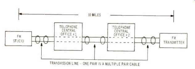
Fig. 1--Showing a straight-through audio transmission line connection.
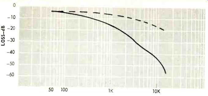
Fig. 2--Dashed line shows loss in 4-mile section of 22-gauge cable. Solid
line shows loss in 10-mile section of 22-gauge cable.
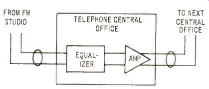
Fig. 3--Audio transmission line with equalizer and amplifier replacing the
straight-through connection in the telephone central office.
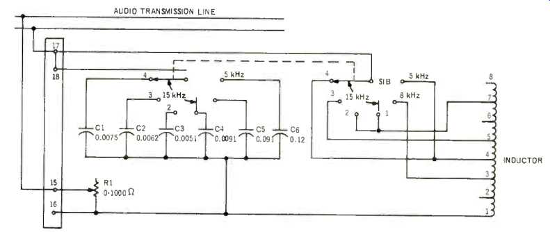
Fig. 4--Showing a schematic of a line equalizer.
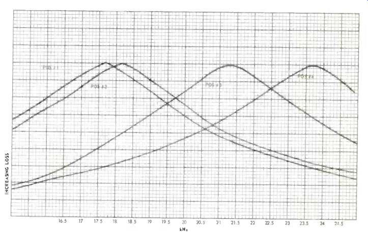
Fig. 5--Equalizer slopes for 4 kHz switch positions.
The equalizer shown in Fig. 4 uses a parallel resonant circuit. Below the resonant frequency, the reactance is inductive and, hence, according to the formula for inductive reactance (XL = 2 pi FL) the equalized loss increases as the frequency decreases. Since the equalizer acts as a variable resistance bridged across the cable pair, it introduces more loss at the low frequencies than it does at the high frequencies.
Also, the lower series resistance introduced by R1, the greater the amount of equalized loss provided. As the frequency increases, the inductive reactance increases. The resistance of RI now has less equalizing effect as the inductor and capacitor approach resonance. Therefore, the equalizer introduces less loss at the higher frequencies. The resultant frequency of the equalizer is designed to be sufficiently above the highest equalized frequency so as to provide the proper slope as indicated by Fig. 5.
The amount of equalization that has to be provided in the first section of the circuit, according to Fig. 2, is 18dB. At the studio, all frequencies from 50 Hz to 15,000 Hz, in 100 Hz steps, are transmitted at 0 dB over the circuit to the first central office. Here the equalizer is adjusted by first selecting the proper 15 kHz position. This is done by experimenting to find out what contour most closely fits the loss of the cable pair. Now R1 is adjusted until the loss of the equalizer is equal but opposite to the loss of the circuit. Figure 6 indicates the result when this adjustment is properly completed.-The result of this equalizing process is not only a flattening of the frequency response but also a drop in overall level. This drop in level is the price which must be paid to achieve a flat frequency response.
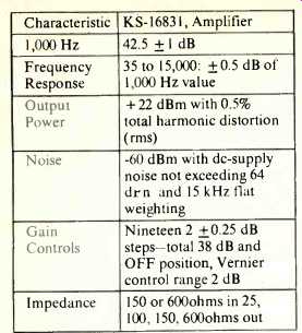
Table A--Electrical characteristics of a solid state program amplifier,
which compensates for circuit and line loss.
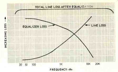
Fig 6--Equalizer effect on total line loss.
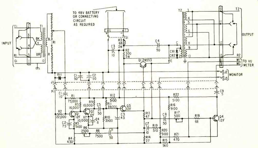
Fig. 7--Showing a schematic of a program amplifier.
Amplification
The next process is to introduce sufficient gain at this point to compensate for circuit and equalizer loss and leave the first central office at a level of 0 dBm. (dBm indicates 1 milliwatt developed into 600 ohms.) Located in telephone offices are amplifiers associated with line equalizers. Figure 7 is a schematic of a solid state program amplifier; Fig. 8 is a picture of the current version. Table A lists some of the amplifier specifications.
A brief discussion of a few of the characteristics might be in order. The maximum gain of the amplifier is 42.5 + 1 dB, which indicates this is not a particularly high gain device. The reason for this is the level of the input signal is normally not lower than -20 or -25 dB. If the input signal was very low-the order of-35 or -40 dB-the signal-to-noise ratio would be so low as to make the signal unusable. Additional gain in this case would serve no useful purpose. The maximum output power is -22 dBm or 158 milliwatts.
This figure may seem unusual until certain considerations are reviewed. The normal average power of the audio signal leaving the studio and all other points which contain gain devices is 0 dBm or 1 milliwatt. Higher output levels would cause interference to be introduced into the other circuits in the cable. Lower output power would cause the signal-to-noise ratio to be poor at the receiving end of the circuit, as a result of low received power. A 0 dB transmission level is a compromise which allows the best results to be obtained, from both a signal-to-noise ratio and an interference standpoint.
Dependability is a prime requirement in telephone company equipment. Program amplifiers are no exception. As a rule, the equipment is turned on when it is installed and tested and never turned off except for maintenance. Thousands of these amplifiers have been performing successfully throughout the country for five or more years, which is a credit to the design and manufacture of this equipment.
The operating voltage for the amplifier is 48 volts d.c., which is obtained from central office batteries. In the event of a commercial power failure, the equipment still operates because the central office batteries are charged independently of commercial power. Jacks are associated with the equipment so that, in case of a failure, a spare amplifier can be patched (inserted) into the circuit in a few seconds. Monitor jacks are provided to check the quality of the circuit if an abnormal condition does exist.
It now becomes quite apparent what has been accomplished in the first section of the circuit. Transmitted from the first central office is a bandwidth of 50 to 15,000 Hz ± 1 dB at a level of 0 dBm. The noise level will be below -67 dB and the distortion will be below 0.4 percent. In effect, the studio has been moved four miles closer to the transmitter as far as the audio output of the first central office is concerned.
The type of circuit that has been described is known as a local program circuit. These are relatively short in length, possibly up to about 30 to 40 miles. In this situation, there could be a maximum of eight amplifiers in series strung along the circuit. The limiting factor as far as the number of amplifiers in series is the distortion contributed by each. With this many amplifiers in series, a reasonable distortion factor is 1.5 percent. Where very long program circuits are involved, such as coast-to coast networks, this technique is not used. Microwave radio or wire carrier systems would be used in these cases. Briefly, in these systems, the audio band is translated to higher frequencies and transmitted as sidebands in the radio frequency spectrum.
The next section of the circuit shown in Fig. 1 is from the first central office to the second central office. The same techniques are used to equalize the second and the remaining sections of the circuit. It is important to know, however, that the audio oscillator remains at the studio and transmits the test frequencies through each equalized section to the next section. With this arrangement, any residual discrepancies in one section can be remedied in the next section or sections. It is important, however, that each section, as far as practical, should be equalized to not only meet but exceed the circuit requirements.
The last section of the circuit, which is from central office number three to the transmitter, is treated differently than the previous sections. An equalizer will be located at the transmitter but an amplifier probably will not be, unless this section is long and, consequently, the received audio level low. The signal-to-noise ratio at the transmitter determines the need for amplification at that location. As an example, if the equalized level is -18 dB, what could the maximum signal-to-noise ratio be? The normal sending level at the studio for program material is +8 VU (volume units) with a peak factor of + 10 VU. (Peak factor indicates the maximum amplitude the signal will momentarily reach). This means the maximum level is + 18 VU. Now if the equalized loss in the last section is 18 dB, the peak level would arrive at a level of 0 VU. If the inherent circuit noise was -60 dB, the signal-to-noise ratio would be 60 dB. Of course, for signal levels less than the peak value, the signal-to-noise ratio would be less.
Stereo Considerations
When the program material is in stereo form, two of the facilities previously described are required. This type of transmission necessitates added specifications comparing the two transmission media. As indicated, the frequency response in each channel shall be ± 1 dB from 50 to 15,000 Hz. The added specification requires the transmission frequency characteristics of the two channels be within 0.5 dB of each other anywhere in the specified audio range. If this requirement is met, the monophonic listener will receive a satisfactory signal. A difference in electrical length between two transmission facilities results in differential phase shift. If one path is slightly longer than the other electrically, the two signals will add vectorially at the receiving end. Figure 9 represents an extreme case of differential phase shift. The signal which traverses the longer path requires a greater time to reach the end of the circuit. The worst possible condition would result if the two paths differed in electrical length by 180 degrees, which is a half-wave length for a particular frequency. As would be expected, this frequency would be greatly attenuated. Differential phase shift between two circuits increases as the frequency is increased because a slight difference in length can represent an appreciable part of a cycle. As a rule, differential phase shift between two circuits used for stereo transmission is quite small and if the requirement can be met at 15,000 Hz, it will be met in the rest of the audio band.
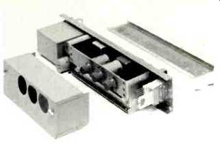
Fig. 8--Showing an audio amplifier and jacks.
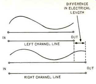
Fig. 9--Showing differential phase shift, with the left-channel line shorter
than the right-channel line.
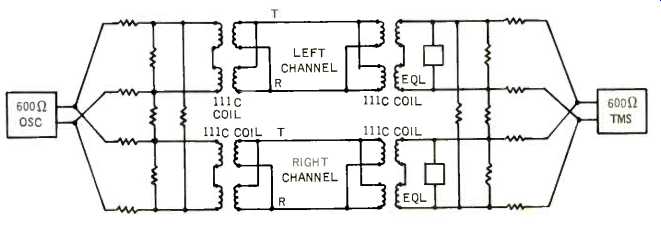
Fig.10--Arrangement for measurement of differential phase shift in stereo
channels. (TMS is transmission measuring set.)
In order to have negligible differential phase-shift, the two circuits must be completely identical in all respects. Both circuits should be in the same cable in all parts of the transmission facility. Identical amplifiers must be used and installed at the same locations. Equalizers must be of the same type and installed at identical locations.
The test arrangement used to check for differential phase shift is indicated in Fig. 10. At the transmitting end, the oscillator is adjusted for an output of 10 dB at 1 kHz. The received level should be equal to the normal received level plus the loss of the resistance network which is 15.4 dB. If this requirement is not met, a frequency check is made. When the differential phase shift is negligible, the response characteristic of the combined circuits should be ± 1 dB from 50 to 15,000 Hz. If one of the circuits is reversed, the two signals will be 180 degrees out of phase and the received level will usually be 20 to 30 dB lower than expected.
Minor discrepancies, where the response at the high end is out of limit, are due to slight accumulated differences in the make-up of the two circuits. This is generally quite easy to remedy.
This is just a brief look into the current technology of audio transmission lines. Many more engineering considerations are involved which we haven't covered. The basic concepts that were examined do give an accurate picture and should give the reader a good insight in this one small facet of audio techniques.
(adapted from Audio magazine, Feb. 1971)
Also see:
= = = =