by Jeffrey H. Johnson [Braun AG Frankfurt, W. Germany]
The story is told of the English child during the war who, on learning of an impending bread shortage, remarked that this wouldn't bother him as he always ate toast. Something of the same outlook has all too often been evident in the attitude toward the amplifier-loudspeaker interface. We measure amplifiers with well-defined resistive loads, but we listen with loudspeakers, and loudspeakers present anything but a constant, well-behaved load to the amplifier. This can lead to a number of problems, and it is becoming widely recognized that an amplifier which "works just fine" on the test bench may not perform so well in actual operation. To see what some of the effects of non-ideal loads on amplifiers are is the purpose of this article.
The Loudspeaker
Loudspeaker manufacturers specify a nominal or "rated" impedance for their products, usually 4 or 8 ohms. This specification is not without value, but we shouldn't forget that the impedance of a loudspeaker actually exhibits considerable variation with frequency. Partly this is determined by the designer's choice of crossover network parameters, etc., but it is also to some extent inherent in the physical principles of operation of the loudspeaker mechanism itself.
Figure 1 shows the measured impedance of a typical three-way air suspension system rated at 4 ohms.
Now, at first glance, it might seem that these impedance variations would be very undesirable from the standpoint of the power available from the amplifier. Since an amplifier is very nearly a constant-voltage source, the power output is inversely proportional to load impedance; the higher the impedance, the smaller the available power. For example, if the unit shown in Fig. 1 is driven at 6.32 V--or 10 W into the rated 4 ohm impedance--a power meter would show that the actual power would vary from about 11 W to about 1 W, depending on frequency. This might seem highly undesirable, but in fact it is not. Loudspeakers are designed for flat frequency response with a constant drive voltage, not constant power. There is no problem here, except that amplifier meters labeled in watts are meaningless. (For a further discussion, see refs. 1, 2, 3.) The problems caused by impedance variations come from a different direction, namely from the fact that an impedance which varies with frequency exhibits a reactive, as well as a resistive, component. A reactance is non-dissipative; it can only store energy, not put it to use. Such stored energy is unavailable for conversion into acoustical energy. What's worse, this stored energy must go somewhere, and that somewhere is back into the amplifier, where it can cause trouble.
Before we look at what some of these troubles are, we need to take a moment to clarify some terminology. Impedance is a complex quantity; that is, it has two dimensions, not just one. We can express this by saying that it has a real (or resistive) part and an imaginary (or reactive) part, and write this as Z = R ± jX where R is resistance and X is reactance. A very useful alternative expression is to ive the magnitude (or modulus) of the impedance: |Z| = √ (R^2 + X^2) . The other dimension is then expressed as a phase angle:
L Z = tan -1 (X/R).
What we usually offhandedly call "impedance" is actually only the magnitude of the impedance: to be completely accurate we should also give the phase angle. The impedance in Fig. 1 is thus both curves taken together. Habitually speaking of the magnitude only makes it easy to overlook the reactive component.
Small-Signal Effects
Reactive loading can affect both the large-signal and the small-signal performance of an amplifier. The small-signal effects have to do chiefly with the feedback stability and the dynamic response of the amplifier.
An amplifier can be modeled by a forward gain path Avon with an internal impedance Zo, enclosed in a feedback loop giving a closed-loop overall gain of Avon (Fig. 2) (Zo here should not be confused with the output impedance of the complete amplifier, which is Zo divided by the loop gain.) For stability the phase shift at unity loop gain must not exceed 180°, and for satisfactory dynamic (transient) response, some phase margin is necessary, limiting the loop phase shift to 120° or perhaps 135°. In terms of the familiar Bode plot, Fig. 3a, this means that the curve of the forward gain must intersect the curve of the closed-loop gain with a slope not much greater than 6 dB/octave, and all higher breakpoints must lie some distance above this frequency.
The feedback voltage is taken from the junction of Zo and the load, point X in Fig. 2. Zo, which may be comparable to the load impedance depending on the circuit configuration, forms a voltage divider for the feedback in conjunction with the load impedance. Suppose now that the load is inductive, so that its impedance increases with frequency. Unless Zo is quite small, this means that the feedback voltage will also increase. With luck, this can provide a degree of lead compensation, but more often the result is that the loop bandwidth is extended so that higher frequency poles begin to contribute to instability, as depicted in Fig. 3b. Alternately, a capacitive load will tend to roll off the feedback with increasing frequency, and so the slope of the forward gain curve is increased and instability results (Fig. 3c). As if this were not enough, in many circuits Zo is not constant but rather increases at higher frequencies due to hfe falloff in the output transistors, etc. Zo will thus have an inductive component, and should the load be capacitive, a second-order LC filter will be formed for the feedback signal, contributing an additional 12 dB/octave rolloff. This leads to oscillation. Often a fairly small capacitance (10 nF to 0.1 µF) will be more troublesome than a large capacitance, since the latter may spread the poles farther apart and give a less rapid rolloff.
The cure for these woes is the addition of load isolation or stabilizing networks to the amplifier output. The simple RC network in Fig. 4a loads down the amplifier at high frequencies, avoiding the situation of Fig. 3b with inductive loads (which are typical of moving-coil loudspeakers), and with the rise in Avon which some configurations exhibit without load. A more thoroughgoing method is the use of the LCR network. A series inductor with rising impedance at higher frequencies is added to prevent capacitive loads from loading down the amplifier too much. The preferred form of this network, Fig. 4b, can be made to effect a smooth transfer of the amplifier from the external load to the resistor R at a suitable frequency above the audio range (Ref. 4). Load isolation networks are sometimes accused of ringing, but with proper design this is not so; most of the ringing is attributable to reduced feedback phase margin in the amplifier.
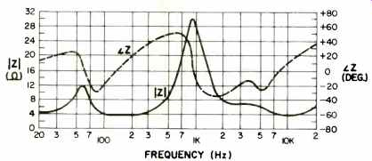
Fig. 1-Impedance of a typical loudspeaker system.
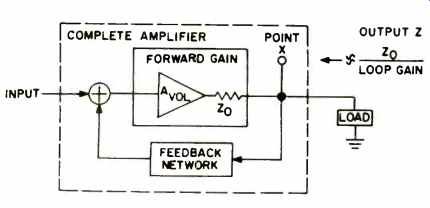
Fig. 2-Model of a power amplifier.

Fig. 3-Bode plots for (a) resistive load, (b) inductive
load, and (c) capacitive load.

Fig. 4-Load isolation networks, (a) RC and (b) LCR.
The small-signal effects are manifested mostly at frequencies well above the audio range. The nature of the loudspeaker load is consequently quite important in this region also. Loudspeaker impedance is usually measured only to 20 kHz, but for some time now one manufacturer has been measuring all new designs out to 1 MHz after it had been discovered that an unexpected impedance dip around 200 kHz had been causing problems with a certain amplifier.
Large-Signal Effects
The major difficulties arising from reactive loading are associated with the large-signal area. Unlike the small-signal case, where the amplifier as a whole is involved, the large signal effects are confined almost entirely to the output stage.
One of the most important effects of reactive loading is its influence on the power dissipation in the output devices of an amplifier. Probably the best way to see how this happens is to examine the load line, which is a plot of VcE and lc for a specified load.
If the load is resistive, the load line will consist of straight line segments as in Fig. 5b (here, and in what follows, an ideal class-B circuit is assumed). The line 1-2 represents all values of VcE and lc during the "on" half-cycle, and the line 1-3 shows that lc = 0 during the "off" half-cycle. The slope of the line 1-2 is determined by the load; if the solid line represents 4 ohms, for instance, the dashed line would show 8 ohms.
An important property of the load line graph is that it also implicitly shows the power dissipation of pr in the output device, since it relates VCE to lc and pT = VCEle. During the "off" half-cycle, pT is obviously zero. During the "on" half cycle, piis small when the output voltage Vo is near zero (point 1 in Fig. 5b). As the output voltage begins to increase, current flows into the load and lc increases. At first pT increases, but since VcE decreases as Vo increases, pT begins to fall, and when the crest of Vo is reached (point 2 in Fig. 5b) pT is again very small. The overall dissipation is thus comparatively small, and the operating conditions of the output device are quite favorable.
The situation is much different if the load is reactive. In a resistance, current and voltage are in phase; but in a reactance, the current and voltage are displaced from one another by the amount of the phase angle, and the minima and maxima of the current and voltage waveforms no longer coincide. If such a load line is plotted, the resulting curve is not a straight line but becomes elliptical. As the phase angle increases, the ellipse becomes broader (Fig. 6). A comparison of these elliptical load lines to the resistive case yields some unwelcome facts. Consider the point of zero V0, where VCE = V. For a resistive load, pT is zero (point 1 in Fig. 5b), but for a reactive load there is a significant flow of lc at this point, and hence considerable dissipation. Or take the "off" half-cycle; here again there is a substantial flow of lc in the reactive case compared to zero for a resistance. This is particularly undesirable, since the combination of high VcE and high lc can initiate secondary breakdown, resulting in a catastrophic destruction of the output transistors.
Additional insight can be gained if the curve of the maximum permissible dissipation-the "safe operating area" (SOA) curve-is added to the diagram. This is done in Fig. 7.
The resistive load line (a) remains comfortably within the SOA. But a reactive load of the same impedance magnitude (b) fills and even somewhat exceeds the SOA. Reactive load lines in general use the available territory less efficiently; they bulge out just about where the SOA curve dips inward.
It is a little difficult to get a quantitative picture from the load line diagram, so in Fig. 8 the dissipation pT has been plotted over one complete cycle, normalized to a peak output of 1 W (or 1 VA). The dissipation is seen to increase substantially as the load phase angle increases. With a purely reactive load (90°) the maximum pT is over five times as great as for a resistive (0°) load. Integrating or averaging pT over time gives the average dissipation pT, which determines the heat sink requirements of the amplifier. This is shown in Fig. 9, with a resistive load taken as unity. Here again there is a significant, if not quite so dramatic, increase in dissipation as the load becomes more and more reactive.
It is now time to introduce a complicating factor. So far, operation at full output has been assumed, but in fact the dissipation is a function of output level. We can include this factor by introducing a "drive factor" k, which varies from 0 to 1 (or 0 to 100 percent). Note that k is in terms of voltage, not power. The dissipation as a function of k is shown in Fig. 10. For a resistive load, the greatest dissipation occurs at k = 63 percent output (40 percent of maximum power output). As the load becomes increasingly reactive, the dissipation increases, and the decline in dissipation near full output also disappears.
It should by now be abundantly clear that operating an amplifier into a pure resistive load is far kinder, far less demanding, than is operation into a reactive load like a loudspeaker. And these relationships apply, let it be added, regardless of whether the output devices used are tubes, transistors, or FETs. To put it another way, an amplifier which is to operate without difficulty into highly reactive loads must be more conservatively designed than would be expected on the basis of purely resistive loading. It must also be borne in mind that the efficiency of real-world amplifiers is less than the ideal case assumed in this discussion.
And speaking of real-world situations, it ought to be noted that this discussion has tacitly assumed sinusoidal signals. For a variety of reasons, such signals have great usefulness in analysis, but they don't correspond very closely to either speech or music. Since the energy content of pro gram material is generally less than a sine wave of equal peak amplitude, the dissipation will in many cases be less than the curves we have seen would suggest. Unfortunately, it is simply not possible to say how much. There are random signals which can model program material quite well, it is true; but strictly speaking impedance is defined only in the frequency domain, and the only signals which would not involve treating a band of frequencies are the exponential and the sinusoid. And once we have to look at a band of frequencies, the precise nature of the load (its impedance versus frequency) would have to be specified, making a general solution impossible.
A Special Case
Before we leave the subject of output stage dissipation, there is an interesting special case that ought to be considered. So far we have allowed the phase angle to vary while holding the magnitude of the impedance constant. A different picture emerges if, instead, we require only that the real part of the impedance remain constant. This is equivalent to saying that the magnitude of Z is allowed to increase as we increase the phase angle, and is shown by the dash-dot line in Fig. 11. The dissipation in this case is shown also in Fig. 11.
The solid curve represents the worst-case dissipation, obtained by letting k be whatever value gives the greatest dissipation. The result is interesting; the dissipation with any arbitrary reactive load under these conditions never exceeds the value of dissipation observed for a resistive load.
In fact, for highly reactive loads (over about 51°), it actually is less. We saw earlier that for reactive loads, the dissipation was greatest for k = 1, and this condition is shown by the dotted line. Here again the worst-case resistive load dissipation under these conditions would never be greater than it would be for a resistive load equal in value to the minimum real part of any complex load. The significance of this will be discussed later, for it forms the basis for a rationalized loudspeaker impedance rating.

Fig. 5-Load line graph.

Fig. 6-Load lines for several load phase angles.

Fig. 7-Load line graph with transistor SOA curve, (a) resistive
load and (b) reactive load.

Fig. 8--Instantaneous collector power dissipation over
1 cycle of output waveform.

Fig. 9-Average collector power dissipation as a function
of load phase angle.
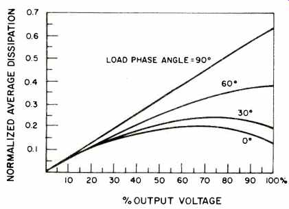
Fig. 10-Average dissipation as a function of drive for
several load phase angles.

Fig. 11-Average dissipation as a function of load phase
angle for constant real part of load impedance.

Fig. 12-Protection circuit characteristics, (a) threshold
curve, (b) with shorted output, and (c) with capacitive load.
The Protection Problem
Another important set of large-signal problems springs, somewhat ironically, from what ought to be a good idea, output transistor protection circuits. The kind of circuit which causes problems seeks to clamp 1 to some value which is a function of the VCE at that instant. Such a circuit, whose threshold characteristics are shown in Fig. 12a, permits the SOA to be nearly fully utilized. A short on the output is clamped as in Fig. 12b, and a purely capacitive load is prevented from exceeding safe limits as in Fig. 12c.
Things are altogether different if the load happens to be inductive. Should the protection circuit be activated in this case, an annoying and potentially dangerous very loud popping sound results. These are the notorious "flyback impulses" illustrated in Fig. 13. The impulses are usually short (tens of microseconds) but of considerable amplitude. Since they contain large amounts of high-frequency energy, damage to tweeters is not unknown. These impulses can occur under seemingly unobjectionable conditions, for example when the magnitude of the load impedance is fairly high and hence the amplifier is only lightly loaded. All that is required is that the load be inductive (i.e., the impedance is increasing with frequency) and that it activate the protection circuit at some point.
Such flyback impulses come neither from the load nor from the amplifier alone, but rather from the combination of the two. The ultimate culprit is the negative slope of the protection circuit threshold. When the current flow into the load is stopped by the clamping action of the protection circuit, the tendency of the inductive load to produce a reverse-polarity voltage forces the protection circuit into even greater limiting. Suppose the output were positive-going at some point, and so VcE were decreasing. If now the current into the load is clamped, the sense of the resulting load voltage will be negative-going. This implies an increase in V that in turn reduces the current clamping level to a smaller current. A regenerative situation exists, and the end result is that the output voltage of the amplifier tends to slam into the clipping region with the opposite polarity. If one such event does not dissipate the energy stored in the load, several pulses may follow one another in rapid succession.
A number of solutions to this problem have been advanced. The basic idea is to avoid having a negative-slope threshold at signal frequencies. One approach places large capacitors in the protection circuit to slow it down ("delayed limiting"), avoiding a regenerative situation. Another method is to use pure current limiting. A glance at the SOA curves shows that this places heavy demands on the output transistors, even when the current limit is made a slowly varying function of signal level. For this reason, paralleled heavy-duty output transistors must be used. The ultimate expression of this line of attack is to use a great many, very rugged transistors in the output stage so that protection circuits can be eliminated entirely. (Tube amplifiers, of course, fall naturally into this category, since tubes can withstand very large short-term overloads.) And finally there is the "solution" of simply making the protection threshold larger, but leaving the output stage as is, on the assumption (or hope) that the overloads encountered in "normal use" will be small enough not to destroy the poorly-protected transistors.

Fig. 13-Flyback impulses with inductive load.
The Practical Conclusion
We have seen some of the effects that reactive loads can have on amplifiers, and we have noted some of the problems that can occur. The question remains, what can be done about them? The small-signal problems can be avoided by sound design and thorough verification of an amplifier's stability before the design is released for production. Amplifiers from reputable manufacturers are usually free of problems.
Large-signal behavior is another matter. It would be easy to say that any amplifier should be able to cope with highly reactive loads. But here we come up against economic limitations. Power sells, and to remain competitive, the temptation is very great to design the amplifier for very high power into a resistive load at the expense of adequate and costly "elbow room" for operation into reactive loads.
One possible solution would be for prospective purchasers to become more aware that the usual power rating per se is only a part of the story. The test reports in the several hi-fi magazines could be of real service here by including reactive load measurements. Heavy capacitive loading has often been used, but inductive loading seems conspicuously absent. A reasonable approach would seem to be to use a set of loads at each rated impedance and at several frequencies. These could be 1) a real load R equal to the magnitude of the rated impedance Zr ; 2) an inductive load ZILI = 2Zr Z +60°, and 3) a capacitive load Z(c) = 2Zr L, 60°. (In other words, R + j0 and R ± j 3X where R and X equal Zr at the frequency of measurement. Proposals of this kind have appeared in the literature (Refs. 2, 5). Another very worthwhile endeavor would be a clarification of the rather nebulously defined "rated impedance" applied to loudspeakers. The most logical approach would be to specify the minimum value of the real part of the loudspeaker impedance, as suggested by Pramanik (Ref. 6). We have seen that the amplifier dissipation with reactive loading will not exceed the dissipation observed with the minimum real part of the impedance. Accordingly, such a specification represents a useful and meaningful measure of the loading produced by the loudspeaker on the amplifier.
Since this specification would not in itself alert a prospective user to possible protection circuit problems in the case of a highly reactive loudspeaker, there would continue to be a need for impedance data, in reviews if not in spec sheets.
Such data should include the angle as well as the magnitude of the impedance, or, as in Audio, the real and imaginary parts.
These proposals are suggested as possible ways to avoid or at least minimize some of the problems we have seen in connection with the amplifier-loudspeaker interface. It is hoped that in the discussion, some light was shed on the origin and nature of the problems as well as on some of the possible solutions. The ultimate resolution of these problems depends, however, on the user. Those who use amplifiers must become aware that presently used specifications do not tell the whole story, and be ready to insist on complete specifications. And perhaps we should also be content with an amplifier that appears a little less powerful on paper, but which makes music come alive through a loudspeaker and does so reliably and without fuss.
Acknowledgements I would like to thank all those within the industry with whom I have discussed these problems. For particularly interesting and illuminating discussions I would like to thank Peter Walker of Acoustical Manufacturing (Quad), S. K. Pramanik of Bang and Olufsen, and Gerry Margolis of JBL; and for bringing to my attention the "delayed" protection circuit I thank J. H. Michel of Gerätewerk Lahr (Thorens/EMT).
References
1-G. J. King, Hi-Fi News and Record Review, Dec. 1976, p. 87.
2-J. H. Johnson, "Realistic Specifications of Amplifier Output," delivered to AES 56th Convention, 1977; AES Preprint 1201.
3-S. K. Pramanik, "Specifying the Loudspeaker-Amplifier Interface," delivered to AES 53rd Convention, 1976; AES Preprint.
4-A. N. Thiele, "Load Stabilizing Networks for Audio Amplifiers," Journal of the AES, 24:1 (1976), p. 20.
5-P. J. Walker, Letter, Wireless World, 81:1480 (Dec. 1975), p. 568.
6-S. K. Pramanik, Letter, Hi-Fi News and Record Review, Mar. 1977, p. 83.
(Audio magazine, Aug. 1977)
Also see:
How Valid is the FTC Preconditioning Rule? (Sept. 1975)
20,000 Watt Home Hi-Fi (Apr. 1976)
= = = =