..
[adapted from article by J. SELMER JENSEN and S. K. PRAMANIK, Audio magazine, Aug. 1984].
J. Selmer Jensen is a freelance designer associated with Bang & Olufsen in Struer, Denmark, while S. K. Pramanik uses his engineering background in long-range planning for the firm.
= = =
Not all of a tape recorder’s bias comes from the bias oscillator—some comes from the signal being recorded. HX Professional lets that work for, not against, the requirements of good recording.
This story has many examples of how a true and deep under standing of a physical phenomenon has been found for the first time through an attempt to solve an apparently unrelated problem. Then, when the problem is solved through this new understanding of its fundamentals, the solution seems so obvious that one wonders why no one thought of it before. And often, when the solution is implemented, it leads to improvements in areas not thought of when the problem appeared, or even when it was solved. All of this applies to the discovery and implementation of the HX Professional tape recording process.
The problem whose solution largely contributed to the invention of HX Professional, while unusual, was not unknown. A quick, accurate, and cost- effective method for fine-tuning cassette recorders was needed for the assembly line. What was thought to be just such a method for adjusting bias and equalization to get flat frequency response was the use of a multi-tone, or comb-frequency, signal.
Such a signal consists of several sine-wave components of different frequency, all at the same level, mixed to form a composite test signal, as shown in Fig. 1A. When this signal is recorded and played back, it should be a simple matter to monitor the output on a spectrum analyzer and make adjustments so that the level of each frequency is equal, as in the input signal. When the adjustment is complete, the recorder would presumably be set up for flat frequency response.
The only problem with this method is that it does not work. No matter how carefully a recorder is adjusted using a comb-frequency signal, conventional frequency-response measurements on the same machine yield a curve some thing like the one in Fig. 1 B. Tape saturation (the condition when tape is magnetized to its uppermost limit so that no further increase is physically possible) leads to a similar result. But, since the same thing happens at low recording levels, any suggestion of tape saturation as the cause has to be discarded. This effect is not confined to any particular recorder or tape formulation, but may be easily reproduced on any standard machine, whatever its price, quality or specifications.
Obviously, the reverse is also true. A recorder set up to give a flat frequency response using a standard sine-wave signal gives a response which looks like Fig. 1C, if tested with a comb- frequency signal. Since speech and music signals are almost never a single frequency, but consist of combinations of large numbers of tones, more like a comb-frequency signal, the frequency response recorded on any normal recorder with real-life signals also looks more like Fig 3. The amount of deviation from flat frequency response depends on the high-frequency con tent of the audio signal and is constantly changing. The error that is produced may be called dynamic frequency-response error. This error is also not confined to any particular kind of recorder, but may be reproduced on any standard machine.
To understand what happens, it is necessary to go back to fundamentals and examine the physical properties of tape and the recording process itself.
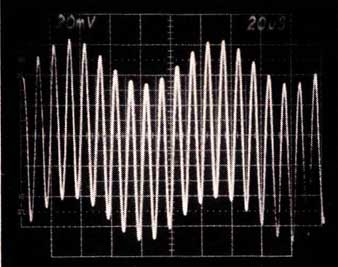
Fig. 1—Theoretically, adjusting a tape deck for flat record/playback response
with a comb-frequency signal (A) should result in flat response. In practice,
it yielded a peaked curve (B) due to dynamic biasing. On a deck set up for
flat response, comb-frequency response declines at higher frequencies (C).
The Physics of Recording
Magnets are known by most people as pieces of metal that attract anything made of iron and are attracted to or repelled by other magnets. But magnets are also useful pieces of hard ware, forming the basis for (among other things) motors and electrical generators—and for magnetic, or tape, recording.
If a current is passed through a coil, a magnetic field (or flux) is created around the coil, similar to the magnetic field created by a permanent magnet. The strength of the field depends on the amount of current, the number of turns of wire in the coil, and other factors. Obviously, the strength of the field that is generated can be regulated by controlling the electric current in the coil. If a suitable magnetic material is held in the flux, it will become magnetized, to a degree that depends on the strength of the flux passing through the magnetic material as well as on the properties of the material itself.
Conversely, if a magnet is moved near a coil of wire, a generated current can be taken from the coil. The amount of current depends on the strength of the magnet, its distance from the coil, the number of turns of wire in the coil, and so on.
These two fundamental facts are the basis of all magnetic recording and reproduction and, in the consumer field, of recording on and playback from cassette tape.
Recording is the process of creating a tape magnetized along its length to a degree which varies exactly as the sound signal received by the micro phone. The microphone converts the sound it receives into an identical electrical signal, which is amplified and fed to the recording head in the recorder. In the recording head, the current passes through a coil, while the tape, of a suitable magnetic material, moves past the coil. The flux generated by the coil magnetizes the tape to a level proportional to the signal so that the audio signal gets recorded.
Similarly, during playback, a tape with the recorded audio signal passes by the playback head, generating in that head’s coil an electrical signal similar to the pattern of magnetization on the tape. With luck, the voltage from a playback amplifier connected to the head will be an exact replica of the audio signal that was originally recorded. When amplified and fed to a loud speaker, the reproduced sound will then be exactly like the original sound received at the microphone.
Although these are the basic physical laws of recording, in practice things are a little more complex. A modern cassette recorder is, in fact, quite an intricate piece of machinery, where each part interacts with all the others in a very precise manner. The degree of precision is a measure of the performance of the recorder, which, in a high-quality machine, can reproduce a very convincing copy of the original audio signal.
Recording on Tape
Recording tape is made of a thin layer of magnetic material deposited on a ribbon of plastic film. The magnetic material is not homogeneous, but is formed from millions of tiny particles, each of which is a magnet. The proper ties of these magnets depend on the material of which they are made (such as ferric oxide, chrome dioxide or iron powder) and are the reason for the familiar tape-type designations. Their physical shape and size, together with their density in the magnetic layer, determine the properties of the recording tape. It is important to remember that we are dealing with these tiny magnets, and that the physical laws that apply to magnets in general also apply to these magnets.
For the purposes of this article, we will assume that the playback chain can be made as perfect as we wish, and concentrate only on the process of recording the tape.
The audio signal to be recorded is constantly changing, and if these changes are to be accurately recorded as different levels of magnetization, then the flux must be concentrated at a very small portion of the tape. The coil in the recording head is therefore formed around poles, which focus the recording field at a very thin-line air gap. The tape transport is made so that the tape slides past the air gap at a constant speed. It would thus appear that, provided we can feed an accurate copy of the audio signal to the recording head, we should get the required recording. But again, this is too simple. To understand why, we must look a little closer into the physics of the tiny magnets on the recording tape.
The strength to which a material is magnetized is, of course, related to the strength of the flux to which it is subjected. In turn, the flux generated is related to the current in the coils formed around the pole pieces in the recording head. But in both cases, the relationship is not linear. In other words, the strength of the resulting magnet is not always proportional to the flux, and the flux is not always proportional to the current in the coil.
The relationship between the residual strength of the magnet and the flux is shown in Fig. 2. The curve, derived from a hysteresis loop, shows that, for an increasing flux, the strength of the magnet increases at first at an increasingly rapid rate. Once beyond a certain point, however, the rate of increase slows, and finally magnetization reaches a maximum value above which no further increase occurs. The magnet is then said to be saturated. The important fact is that there is only a small part in the middle of the curve that is a relatively straight line, and it is only in this region that magnetization is proportional to the flux.
If the different magnetization levels required for a recording can be limited to the linear part of the hysteresis curve, an undistorted recording should result. Audio signals are both positive and negative, so recording will normally be made in the nonlinear portion of the curve near the axis. If a separately generated signal, called a bias current, is added to the audio signal, the average level of the audio signal may be raised so that only the straight portion of the curve is used for recording. In the early days of magnetic recording, a constant d.c. signal was used to bias the audio, but for the last 50 years, a bias current consisting of a high-frequency ac. current has been used. This is called high-frequency (or H.F.) bias, irrespective of its actual frequency.
If a very-high-frequency signal is mixed with the audio signal, the sum looks like Fig. 3. The audio looks as if it is riding on the peaks of the high frequency. If the sum is fed to the coils, then the audio signal will be recorded at a higher part of the hysteresis curve, as shown in Fig. 4. If the high-frequency bias is at the correct level, a low- distortion recording is possible.
To obtain the best results, different formulations of tape require different levels of bias, because the shapes of the hysteresis curve for the different tape formulations are not the same. This is why many recorders permit the user to adjust bias for the type of tape being used, or, alternatively, the recorder is factory-adjusted for certain recommended types of tape. Once set, the bias, supplied by an oscillator, remains at a fixed level, which may be called the fixed bias of the recorder.
Bias for the lowest possible distortion is also different for different frequencies. In addition, bias affects other parameters, such as sensitivity and maximum output level (MOL).
Sensitivity is the ratio of the output signal to input signal, with all other variables kept constant. If the input is kept constant and the bias is changed, it will be seen that the output will vary, as shown in Fig. 5. Not only that, but the shape of the curve is different for different frequencies, as shown.
The same is true of MOL, the maximum output level that can be reproduced from tape. Above this level, the magnets on the recording tape are saturated, and distortion increases dramatically if a recording at a higher level is attempted. Again, MOL is dependent not only on bias but also on frequency, as shown in Fig. 6.
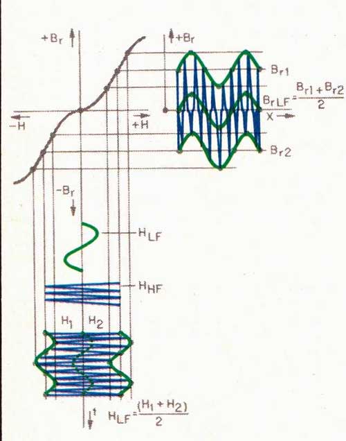
Fig. 2—This transfer function shows the relationship between record-head flux
(“H”) and remanent magnetic field (“B”) when recording without bias. Note how
the curve’s shape alters the relationship between signals of different amplitudes.
These factors are now getting complex, especially if we note that minimum distortion and maximum output do not occur at the same bias level. Of course, we always wish to record at the highest level consistent with acceptable distortion to keep tape noise or hiss as far below the recorded signal as possible. Thus, a correct setting of the fixed bias, while very necessary for good results, is always a compromise between low distortion and high recording level, for both high and low frequencies. For optimum results, set ting fixed bias is best c by an experienced technician using accurate instrumentation, and, in fact, the spectral content of the type of music to be recorded should also be taken into ac count.
The Comb-Frequency Paradox
 Fig. 4—How bias shifts the audio signal to the linear portions of the hysteresis
curve, lowering distortion.
Fig. 4—How bias shifts the audio signal to the linear portions of the hysteresis
curve, lowering distortion.
Now that we know “all” that there is to know about the physics of recording, we are now in a position to solve the paradox of the comb and single sine-wave frequency responses. We saw that bias, as used for recording, is a very high frequency compared to the audio signal. Thus, if we wish to record a bandwidth of, say, 20 kHz, it would be normal to use a bias frequency of five times that frequency, or 100 kHz. The criterion is that the bias frequency must be sufficiently high as to allow the low frequency to ride on the peaks of the high-frequency signal.
If this is so, then bias at a frequency of 10 kHz will be fully adequate to bias an audio bandwidth of 2 kHz, and 1 kHz for 200 Hz, etc. But when the audio signal is a mixture of low and high frequencies, the low frequencies do not know whether high frequencies were put there by the recorder’s de signer to act as bias, or whether they are just a part of the audio signal itself. When a high frequency, whatever its source, is superimposed on a lower frequency, the high frequency will tend to raise the point on the magnetization curve where the low frequency is re corded, just as bias does. Thus, in an audio signal composed of many frequencies, each frequency acts either partially or fully as bias for all lower frequencies.
When the high-frequency part of the audio signal acts as bias, the bias seen by the lower frequencies will be the sum of the original fixed bias to which the recorder was adjusted plus the biasing effect of the higher frequencies. Therefore, bias will constantly change with the high-frequency content of the audio signal, and, for the low frequency, all parameters related to bias (such as sensitivity, distortion and MOL) will change with the high- frequency content in the same audio signal.
That this is true is seen from the case of the comb and sine-wave frequency responses. If the bias in a recorder is adjusted to a flat response with a swept sine wave, then all frequencies see constant bias while the test is con ducted, that is, the fixed bias to which the recorder is adjusted. When multiple frequencies are present simultaneously, each frequency below the highest will be subjected to altered bias, which is the fixed bias plus the biasing effect of all the higher frequencies. As bias changes, the sensitivity for any frequency will not remain the same as before. The output at the different frequencies will therefore change, and the frequency response, as seen on an analyzer, will no longer be flat. In other words, we have dynamic frequency-response error.
It may not be out of place to repeat that this is what happens with all recorders that use fixed ac. bias. This includes not only cassette tape recorders, but also reel-to-reel machines, studio machines and high-speed duplicators, although the amount of dynamic frequency-response error will vary from one type of machine to another and for different tape formulations. The amount of error is related to the ratio between the audio and bias currents fed to the recording head. The smaller this ratio, i.e., the closer the magnitudes of the audio and bias currents are to each other, the larger the error will be.
Active Bias
To sum up the problem, we have seen that the loss of high frequencies when recording at high levels is due less to tape quality than to the fact that there is an increase in the effective level of the bias current when high frequencies are a part of the audio signal. If active bias is too high, then sensitivity at high frequencies decreases, and the output at these frequencies drops. The larger the content of high frequencies, the greater the drop. Once this fundamental principle governing high- frequency performance has been established, the answer to our problem becomes almost obvious. This has been implemented in the recording circuit, HX Professional.
The total bias seen by the low-frequency component of any audio signal, as described earlier, is the sum of the fixed bias and the biasing effect of the high-frequency part of the same audio signal. It will be remembered that it is the immediate value of this sum which determines the recording conditions for the audio signal. It will be useful to use another term for the sum of the bias and the biasing effect of the audio current, and we will call this sum active bias.
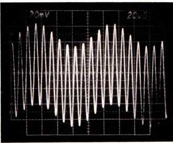
Fig. 3—A low-frequency audio signal riding on a high-frequency bias wave.
Experiments using a high-quality sound source with high treble content and a cassette recorder using ferric tape show that active bias can vary by as much as 6 dB at different parts of the recording. This is equivalent to saying that bias is incorrectly adjusted by that amount, at least for some part of the recording. The consequences are obvious for anyone familiar with the procedure of adjusting bias. The disappointing result, a loss of treble performance—particularly with the less expensive tape formulations at high re cording levels—is most often attributed to poor tape quality, tape saturation or other causes, rather than to a constantly changing bias.
Low frequencies see a uniform level of high-frequency bias, provided active bias is kept constant. This is accomplished when bias from the oscillator is reduced until active bias returns to the level of the “fixed” bias whenever high frequencies are present in the audio signal. The term fixed bias, of course, now loses its original meaning, as bias from the oscillator no longer remains fixed. So we define another term, no-signal bias, which is the bias level to which the machine is set with zero signal at the input, and it is equivalent to fixed bias in a conventional machine. We shall return to this, and see how no-signal bias can be optimized more effectively with the HX Professional circuit.
Keeping active bias constant implies two operations: First, monitoring the active bias continuously, and second, changing oscillator bias as necessary to keep active bias constant.
The black portion of Fig. 7 shows a typical recording circuit in a conventional recorder. The signal output from the recording amplifier is mixed with the high-frequency bias current, typically five times the frequency of the highest audio frequency to be record ed. Bias current or, more correctly, no- signal bias current, is set to the optimum level for the tape in use. The mixed audio and bias current is then fed to the recording head.
What is added to implement HX Professional is a high-impedance monitor for active bias. The ideal place to measure active bias is, of course, at the point where it acts, at the recording head. The sum of the audio and bias currents is first passed through a filter, and the voltage is monitored to deter mine the flux being generated by the head. At this point some wise men will shake their heads and say we should be measuring the current, as it is well known that the flux generated is proportional to the current, and not to the voltage.
While this is theoretically true, in practice such a measurement fails to take into account losses in the magnetic and electrical circuits of the tape head. For various reasons, these losses are not proportional to the current, and magnetization of the tape is therefore also not proportional to the current. This is a failing of certain systems designed to improve recordings, which base the improvement on a measurement of recording current.
So, in the HX Professional system, the voltage across the head is monitored and integrated to give a calculated value of the useful flux generated in the tape head. Flux is actually proportional to this calculated current, as the influence of head losses on the voltage across the head is very small. The calculated value of flux is therefore a very close approximation of the effective magnetizing field. Thus, if the characteristics of the filter are suitable for the purpose (that is, it is designed to reflect the level of active bias accurately and constantly), it can be incorporated into a feedback loop that will keep active bias constant.
The Filter
The characteristics of the filter may be found by experiment. Since we wish to minimize any changes in frequency response caused by the high-frequency content of the audio signal, we may be tempted to proceed as follows:
Using a low-frequency input signal of, say, 200 Hz, bias is adjusted to give the lowest possible distortion of that signal. Then, the low-frequency signal is recorded on tape at a fairly high level, say, 20 dB below the level at which the tape is saturated (that is, 20 dB below MOL). Its output level is measured as a voltage on the output terminals of the recorder. The same frequency is then recorded at the same level, but this time with a high-frequency signal superimposed, let us say 15 kHz, at a level sufficiently low to ensure that saturation does not occur.
When this is done, it will be seen that the output level of the low frequency falls, because sensitivity has changed due to the change in active bias. The amount by which it falls will be seen to depend on the relation between the two frequencies, as well as their relative levels. For this particular case, we can now reduce the bias current until the output of the low-frequency signal returns to the same level as the one it had before any high frequencies were superimposed.
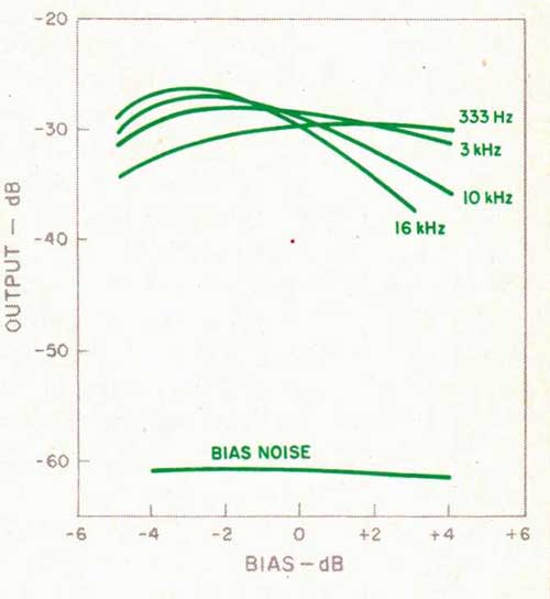
Fig. 5—The relationship between tape sensitivity and bias level varies with
frequency.
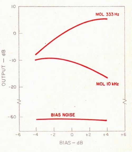
Fig. 6—MOL also differs with both bias level and signal frequency.
When the audio signal contains both high and low frequencies, the highs act as added bias for low frequencies.
We have now achieved the condition, albeit manually, where no change in frequency response occurs due to the presence of the high frequency. The amount by which the oscillator bias needs to be reduced is then the biasing effect of the higher frequency on the lower. This procedure might be repeated for a number of different frequencies, at various input levels, when it should then be possible to work out a mathematical relationship between the ratio of the frequencies and their relative levels.
However, using a filter designed to this relationship does not lead to a flat frequency response. A slightly altered procedure is required, which will give the primary condition of a conventional flat frequency response and consider ably reduced dynamic frequency-response error. The procedure to find the true value of active bias is similar in principle but uses extrapolated points on bias-related parameters as reference, rather than a simple frequency- response parameter. However, if the relationship derived from this procedure is fairly constant at various frequency ratios and relative levels, then a filter for this purpose may be economically constructed.
It is found experimentally that the ‘biasing effect of a sine-wave signal on a signal very close to it in frequency is virtually zero. As one of the frequencies increases, its biasing effect on the lower frequency increases at 6 dB/octave, provided they are both at the same level.
It turns out that the filter we require is one of the simplest among electronic circuits. In fact, it is so close to being a simple filter at 6 dB/octave that any attempt to get a more accurate form, at least for cassette tapes, is superfluous. In other words, if a low-pass filter, passing all frequencies below the highest the machine is designed to re cord, is put into the control loop, the active bias can be correctly set for all audio frequencies. And this setting adjusts itself, by its very nature, to all static bias levels and for all tape formulations.
Once the form of the filter has been determined, our problem is solved. It only remains to construct a suitable circuit that will implement the filter .as part of a feedback loop to control the bias level. For a competent circuit de signer, this really should present no particular problem.
The Circuitry
It will come as no surprise at this point to see the final circuit, which is shown in Fig. 7. As stated earlier, the audio line feeding the recording head is conventional except that the signal is sensed at the head, to derive the signal required for HX Professional. An advantage of measuring at this point is that it allows the audio signal path to, be kept totally free of any manipulation by the HX Professional circuit and therefore free from any possibility of degradation. Further, any necessary manipulation of the signal, such as pre-emphasis or noise-reduction circuits, is automatically taken into ac count when the signal is monitored at this point.
The signal monitored at the head, after passing through an integrator and the filter, is rectified to give a d.c. voltage proportional to the active bias. This is then compared to a previously set reference voltage. The presence of any high frequencies in the signal will alter the level of the rectified voltage by an amount dependent on the amplitude and frequency composition of the signal and the characteristics of the filter. When the rectified voltage changes, it will differ from the reference voltage, and a control signal proportional to the difference is generated. The control signal is used to alter the gain of the voltage-controlled amplifier, which in turn alters the bias current from the oscillator.
The reference is a stable, adjustable d.c. voltage set to a value that gives the required no-signal bias current. The difference between the rectified signal and the reference voltage is used as a control signal to adjust the bias level from the oscillator. It can be seen that in the absence of any audio signal, no-signal bias current at the tape head can be accurately adjusted for any tape formulation simply by changing the value of the d.c. reference voltage. Once this adjustment has been made, the circuit requires no further adjustment or correction.
The bias circuit for HX Professional differs from the conventional in that a voltage-controlled amplifier is placed between a conventional oscillator, which is also used in the erase circuit, and the point at which the audio signal is added to the bias in the recording circuit. This amplifier, as its name suggests, changes its gain under the control of a d.c. voltage to control the amount of bias Current that is fed to the mixer. The d.c. voltage used to control the amplifier is, of course, the signal that is derived from the feedback circuit, which senses the signal at the tape head.
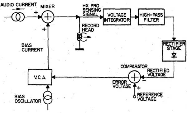
Fig. 7—In conventional recording circuits (shown in black), low-frequency
response can be diminished by the biasing effects of high audio frequencies.
With the addition of the HX Professional circuits (shown in color), bias level
is controlled by the total high-frequency signal (audio plus bias) at the recording
head.
What now happens is that, for an audio signal composed of high and low frequencies, the active bias increases, and oscillator bias is reduced by a corresponding amount. The low frequencies see a total bias equal to the sum of the oscillator bias and the biasing effect of the high frequencies. By definition, and courtesy of the HX Professional circuit, this value remains constant. The high frequencies see the reduced bias from the oscillator, but are far less sensitive to the biasing effect of the high frequencies themselves. In other words, they see a reduced level of active bias.
As we have seen earlier, high frequencies require a lower level of bias for optimum recording conditions than low frequencies do. Thus, the lower oscillator bias is advantageous for the high frequencies in the audio signal, and results in better MOL, besides lowering the dynamic frequency-response error. Together, these two factors lead to a dramatic improvement in the quality of recorded high frequencies, particularly when high recording levels are used. The improvement is more marked on less expensive tapes, but also substantial with the most expensive formulations.
HX Professional also has other ad vantages as byproducts. As mentioned, conventional recorders use a “fixed” bias adjusted to a value which is a compromise between levels that give the lowest distortion at low frequencies and the highest MOL at high frequencies. A compromise is necessary, as the optimum values for these characteristics occur different levels of bias. The compromise is, of course, chosen to be somewhere between these two optimum values.
After implementing HX Professional in a prototype recording circuit, it was realized that the conventional compromise may be considerably reduced. Since the high frequencies take care of themselves, i.e., oscillator bias falls to accommodate high frequencies, no- signal bias may be adjusted close to the optimum value for the best low- frequency distortion. This lowers over all distortion in the recording at the same time that high-frequency recording is improved.
Finally, it was found that the tape overload characteristic for high frequencies, at levels above those where tape saturation begins to occur, is more gentle with the HX Professional circuit. Distortion rises at a slower rate as the normal maximum recording level is exceeded, permitting higher re cording levels and a better signal-to- noise ratio without audible distortion at unexpected peaks in the audio signal.
HX Professional vs. Dolby HX
A description of HX Professional will be incomplete without mentioning the circuit from which it gets its name, Dolby HX. Although the names are similar, as are some of the principles on which the two circuits are based, they are in fact quite different in their aims as well as in implementation, K. Gundry of Dolby Laboratories, the inventor of HX, realized that a wide- band audio signal has a self-biasing effect and that this is part of the cause of high-frequency losses in recording. The problem led him to develop a circuit where oscillator bias, is changed when high frequencies are present in the audio signal, as is done in HX Professional. But his aim was to permit the maximum level of high frequencies to be recorded—in other words, to get the highest possible level of MOL. Hence the name HX, Headroom eXpander system.
However, in order to maximize MOL, oscillator bias must be reduced by more than is necessary to keep active bias constant. Also, a frequency-response error (in a sense opposite that of a conventional recorder, and at an unacceptable level) is introduced due to overcompensation. This was also recognized, and an ingenious correction was introduced.
Since Dolby noise-reduction circuits already measure the high-frequency content of the audio signal, in Dolby HX the same circuit was used to derive a signal to control oscillator bias. In addition, this control signal was also used to alter pre-emphasis to continuously correct the dynamic frequency- response error. The resulting circuit required fairly complex design and adjustment for both the oscillator and pre emphasis to track correctly, and the problem became even greater when using different tape formulations.
Although dynamic frequency response, even with correction, was substantially less accurate than with HX Professional, HX did in fact function marginally better than HX Professional in improving MOL. The reason it ‘did not become more popular was probably because tape recorder manufacturers were not willing to cope with the complexity of the adjustments required for correct operation.
HX Professional was developed at the same time as the Dolby circuit, although independently, but it was re leased later. And it is so fundamental to record technology that Dolby Laboratories not only took part in the final stages of development, but agreed to license the circuitry, on be half of the inventors, to manufacturers not only of cassette recorders but also of other recording devices (such as high-speed duplicators).
This explanation of the function of HX Professional is necessarily simplified in the interests of an explanation of the broad principles at the cost of rigorous detail. The authors hope that readers will take this into account. More exact formulations will be found in the references below.
References:
Gundry, Kenneth, “Headroom Extension for Slow-Speed Magnetic Re cording of Audio,” Preprint No. 1534 (G-2), 64th AES Convention, Nov. 1979.
Jensen, J. Selmer, “Recording with Feedback Controlled Effective Bias,” Preprint No. 1852 (J-5), 70th AES Convention, Oct. 1981.
Jorgensen, Finn, Handbook of Magnetic Recording, Tab Books, Blue Ridge Summit, Pa., 1970.