Analyzing four music selections, this author relates them to amplifier peak power demand, maximum SPL, high-frequency distortion, and, in two cases, sound quality.
SPL tends to be judged on the basis of average power, but it’s the peaks that are amplifier limited. So the higher the peak-to- average power ratio, the lower will be the SPL capability without clipping. And while most music has a significant HF rolloff in average power, HF peaks can be quite strong. In one selection presented here, the peak power at 4kHz and 14kHz is 5dB higher than that at any lower frequency. And, of course, amplifiers usually have the highest distortion at high frequencies and with sharp transients.
I analyzed four musical selections during a sustained maximum-volume segment for peak and RMS voltages—both directly and within ½ octave bands across the spectrum. I plotted the data in relative dB as peak and average power and tabulated it as a percentage of total peak power present within octave bands; the latter allows estimation of an amplifier’s clean HF power capacity requirement.
DEFINITIONS
1. Peak Power
Since amplifiers are rated in average sine-wave power (not instantaneous crest power, which is double), and be cause most of the highest peaks from acoustic instruments look nearly sinusoidal (Photo 1A), it’s consistent and convenient to use the average power (or RMS voltage) in the highest transient half-cycles, averaged or RMS’d over their duration (Fig. 1).
Then,
V_PRMS = V_P/ _/2
This voltage, when squared and divided by some load resistance, results in the average power of the transient.
VRM is the long-term RMS voltage (1.ls averaging time in my measurements), which when similarly processed results in the long-term aver age power. Then V is the ratio of the maximum sine-wave amplifier power needed to the average waveform power. Maximum sine-wave power (half the instantaneous power at the peaks) is used to be consistent with standard amplifier power rating practice.
In this article, the term “peak power” means “maximum sine power,” not absolute peak power (twice as much). So defined, the peak/average power ratio in dB is 20log (Vp/V_RMS). The crest factor (Vp/V_RMS) expressed in dB is 20log (Vp/V_RMS), 3dB higher than the as-defined peak/average ratio.
2. Average Power
Obviously with music this depends on the averaging time. The ear (also the eye) has an integration time of about 1/20 second. Events repeating more slowly than about 20Hz are resolved as a time sequence, or rhythm. So a power averaging (or V averaging for RMS voltage) time of ½os is a lower limit, and this duration also includes one cycle of the lowest audio frequency.
But in observing the output of an RMS to DC converter with variable averaging time constant, ½o or even 1/20th sec. allowed too much LF ripple or “flickering” on the output to obtain stable readings. Also, some peaks would un desirably increase the supposedly aver age result viewed on a meter.
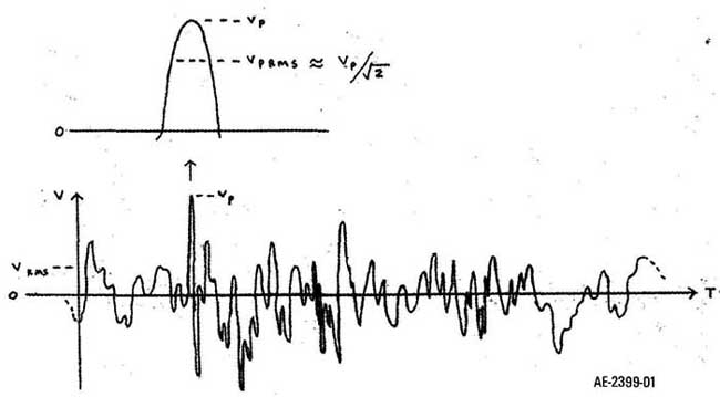
Above: Fig. 1: Definitions.
With average times longer than about 0.5s, readings were stable and didn’t change significantly with longer average times, if the perceived SPL was constant. I then wired the RMS detector for switchable 0.1 or 1.1s averaging times. No reason for the 1.1 figure (resistors and caps on hand, you know). For all but one measurement, I used the 1.1s averaging for RMS voltages.

PHOTO 1: ‘Scope 200mV.
MEDIA SOURCE MATERIAL:
1. Emmanuel Chabrier “España,” Ansermet/L’Orchestre de Ia Suisse Romande, Decca 448 576-2: A very lively piece, recorded in 1964 directly onto two-track tape. Probably not coincidentally, the audio waveforms have high pea1 ratios especially at high frequencies, and the sounds are very dynamic with natural “bite.” Also, the stereo depth puts many modern recordings to shame. (Ask Ed Dell how he likes the Ansermet/Suisse Romande recordings!)
2. Handel “La rejouissance,” HiFi News HFN020: A horn fanfare with (not too loud) fireworks. Even with the latter, strangely, the peaks and peak/aver age ratios were much lower than in Espana. And while the performance was dynamic, the sound seemed muted and the spectrum (even of peaks) was much more rolled off above 2kHz.
3. John Pizzarelli: “If Dreams Come True,” Telarc SACD-63 546: Very well recorded popular song with George Schering on piano.
4. George Strait “All My Ex’s Live in Texas,” MCA MCAD-5913. A great performance and clear recording, except for a highly (studio) boosted 3-18kHz content. Serving as an extreme example of HF peak power demand, the highest peaks (from a rhythmic snare drum beat) are at 4kHz and 14kHz, and at 5dB above the rest of the spectrum. At 14kHz the peak/average ratio is about 25dB, a 316:1 power ratio. About 33% of the peak amplifier power output will be in the 5kHz-20kHz band.
HIGHEST TRANSIENT WAVEFORMS
The high snare drum peaks in George Strait’s recording allowed consistent scope triggering while also showing the complex waveform summation of the multiple instruments playing ( Fig. 2); Photos 1A— present this on different time scales.
Photos 2A and 2B show stereo X-Y cross-plots (Lissajous figures). They aren’t single sweeps as in Photos 1A-C, but 1 exposures where the dense average central regions saturated the film, because high scope brightness was needed to cap ture (some of) the peak excursions.
Lissajous displays also reveal left-right correlation: mono produces a 45° straight line; a 90° shifted L-H sine wave makes a perfect circle, and natural-sounding stereo music generates a round, almost spherical-looking pattern as in Photo 28, from España. This recording has excellent stereo depth and imaging.

PHOTO 1B; PHOTO 1C
TABLE 1: Audio Waveform Properties, 10 sec. Interval Loudest Playing.
Chabrier – Handel – Pizzarelli - Strait


Above: Fig. 2: Test setup, unfiltered audio.
Above: Fig. 3: Test setup, ½ octave filtered audio..

PHOTO 2A; PHOTO 2B:
LONG SWEEP STORAGE SCOPE WAVEFORMS
Photos 3-10 show a single sweep of is (Photos 3-6) and lOs (Photos 7-10) for a steady high-volume segment of the selections. Of note in the George Strait country song in Photo 10 are the repetitive high peaks (containing very high relative power even at 18kHz); these are the snare drum accents.
PEAKS AND AVERAGES OF AUDIO WAVEFORM
The highest peaks, RMS values, ratios thereof (crest factors), and peak! average power ratios are shown in Table 1. For the peaks, the dBm values (re 0dBm = 0.775V RMS, 1.095V peak sine) are calculated for a sine wave with the same peak voltage as the observed musical waveform peak. This is consistent with the stated definition of peak power as the average power within the highest peaks (which most often resemble sinusoidal half- cycles). This is also consistent with the average sine-wave power rating of amplifiers.
1/3 OCTAVE FREQUENCY SPECTRUM
The 1/3 octave filter ( Fig. 3) was stepped through the audio spectrum, noting the highest peaks and RMS voltages at each filter frequency. Results are presented for España in Table 2.
Figures 4-7 show (top traces) the spectrum of the highest peaks, manually plotted from this data; lower traces are the averaged values. Note that with peak power as defined here, the “peak” and “average” traces would be the same for a sine-wave signal.

PHOTO 3; PHOTO 4; PHOTO 5
NOTABLE FEATURES:
1. The most surprising feature is the HF power in the peaks of George Strait’s song (top trace, Fig. 7). I’d bet that someone in the studio cranked up two HF EQs to get peak power at about 4kHz and 14kHz, which is 5dB higher than at any lower frequency.
2. In Fig. 7 only, I plotted the RMS level with 0.1s averaging time in addition to the 1.1s average RMS shown in all four selections. Note that around 200Hz, the shorter-time average nearly equals the peak. This implies a nearly sinusoidal waveform, of nearly constant amplitude within the 0.ls averaging time.
Such a signal can be produced by the upper notes of a bass (and standard) guitar: 200Hz is in the upper range of a bass guitar, where harmonics are most attenuated. Such notes can have nearly sinusoidal waveforms.
3. Note that only in the Handel piece (Fig 5) does the spacing between the peak and average traces stay nearly constant over the whole frequency range. With the other selections, although the average traces roll off at high frequencies, the peak traces roll off much less or actually rise ( Fig. 7), producing a greatly expanded spacing between peak and average at the highest frequencies. This is because most of the peak power in the high treble is from short-duration percussion ac cents (short relative to their repetition time); this low duty-cycle results in ( For example, Fig. 7 at 12kHz) a 25dB peak/aver age ratio (about a 316:1 power ratio).
4. Below about 1.2kHz, the peak/ average ratio in all selections is mostly within a 5-10dB range. Considering just for now the 3dB “crest factor” of a sine wave (twice the average power at the sine peaks), the crest factor of the signals below 1.2kHz is approximately 8-13dB, similar to that of Gaussian noise.

PHOTO 6 – 8
PERCENTAGES OF PEAK POWER IN OCTAVE BANDS
In Table 2, the filtered band peak output voltages were RSS (root- sum-square) totaled; this is valid for uncorrelated signals, such as different frequencies or noise sources. The resuit (1413mV) is within 0.5dB of the 1500mV input peak. Next (not shown), I calculated RSS sums within octave bands and tabulated, in each band, squaring this octave-peak voltage and dividing by the l500mV input peak squared. This result is a power ratio, the fraction of peak signal power present in a particular octave band.
Adding these octave percentages was within the same 0.5dB as with the Table 2 results, of equaling 100% of the signal power; for convenience they were scaled to total 100% in Table 3.
Note that the validity of the calculations depends on different frequency peaks occurring reasonably simultaneously: consider, for example an alternating duet between a bass guitar and a flute, of equal signal voltage for convenience. With this frequency separation, two separate sets of filtered bands will produce alternating, not simultaneous, outputs. So it would be wrong to sum them and expect this to equal the input signal; the bass range and the flute range powers would each be 100% of the input signal power, inappropriately “totaling” 200%. But with these four selections, the sums were within 0.5dB of the input power, so peaks across the spectrum must be occurring reason ably simultaneously.
This is not surprising, since in a musical climax or (especially) a strong rhythmic accent, all the instruments contributing would likely play loudly and in as close timing as possible.
Table 4 shows, for comparison, the octave band average power distribution for the España selection. Note that below about 600Hz the aver age power has a larger fraction than the peak power, but vice versa above 600Hz.

TABLE 3: Percentages of peak audio power present in each octave band. Octave
Band Chabrier
TABLE 4: Percentages of audio power present in each octave band, Chabrier Espana.
Octave Band Peak Power % Average Power %

SONIC EFFECTS OF IM ON HIGH-FREQUENCY TRANSIENTS
With harmonic distortion, even-order is accepted as less objection able than odd-order. Not so for high-frequency TM distortion. Consider a transient—say, mostly occupying an 8-12kHz, BW—of high peak power.
The maximum range of third-order TM products is 2(8kHz)—12kHz, and 2(12kHz)-8kHz, or 4-16kHz. So with enough TM the original transient-signal BW of 4kHz becomes tripled, spread out to a 12kHz BW. Still, within the HF range above 4kHz and of very short duration, a moderate amount of TM could be unnoticeable.
But second-order TM is very different. Here the products are simple frequency sums and differences, and the range of difference products from a continuous 8-12kHz signal band is zero (DC) to 4kHz. Enough second-order TM, or asymmetrical limiting, will produce an audible “spectral downwash,” a crunchy sound extending into the lowest bass. This is why SET amps should not be overdriven.
AMP HIGH-FREQUENCY PEAK POWER
With an amp playing just below clip ping, it’s interesting to know how much of the amp’s HF power capacity (often below normally stated midband power rating) is being used up; how much margin (if any) is there?

PHOTO 10

Figure 4: Spectrum.
The extreme example with top octave studio boost needs the following fractions of peak power in the stated bands: 5% (16—20kHz), 20% (10—20kHz), and 33% (5-20kHz). There could be recordings with even higher percent ages, such as close-miked small bells or chimes, special effects, synthesizers, and so on. Also, SACDs (100kHz response) may contain significant ultrasonic content.
But it seems unlikely for audiophile-quality recordings to have more than one-third of the peak power above 5kHz; the Espana selection has about 16%, and it’s a very (and naturally) brilliant sound.
Flash back to Glass Audio 5/2000, where the Antique Electronic Supply AE-25 “Super Amp” is reviewed. Rated at 15W/channel triode, Charles H. measured only 2.3W at 3% THD at 20kHz (p. 35). That’s 15% of rated power. But even the George Strait recording needs only 5% in the narrower ½ octave 16-20kHz band.
Charles H. measured 19 +20kHz TM at 0.98% with 6V p-p, 8W, an instantaneous crest power of 1.125W, and average power of 0.281W (4:1 ratio, 2:1 voltage crest factor for an equal-amplitude two-tone signal). The ±3V peaks would correspond to a 0.56W single sine wave (at 19 or 20kHz); 0.56W is 3.7% of rated power for 1% TM distortion at 19-20kHz.
Enough trying to mathematically predict the sound: Ken and Julie Ketler, whose many reviews testify to their sonic perceptiveness, gave the AE-25 a generally praise-filled review. One comment possibly relating to this article, comparing the AE-25 with a Valve Audio Lab VAA-100ES 30W p-p amp: “The snares on the bottom drumheads are much more clearly defined with the Super Amp. The difference is particularly noticeable during quiet sections.” Regarding the latter sentence, I would guess that at louder levels the AE-25 runs out of HF power, degrading performance to that of the comparison amp (or the snare drum at louder levels overloaded the recording system or other component).
PEAK POWER VERSUS SPL
Suppose you desire a maximum SPL of 90dB—loud, but not that loud—and your speakers’ sensitivity is 86dB, 1W, 1m. From ten feet away, this would be 76dB with 1W anechoically, but with typical room reinforcement I measured a drop of only 3dB. So at the listening position, each speaker delivers 83dB SPL at 1W. With (generally non-phase correlated) stereo, each speaker needs to deliver 87dB SPL for the desired 90dB example.
This requires 4dB more than 1W, or 2.5W average power per channel.
With the George Strait recording, peak (sine-weighted) power is 42.7 times the average, so 107W per channel is needed for a 90dB average SPL without clipping. With the Handel recording, 33W per channel is needed.
Here’s an extreme example: You heard an orchestra playing Espana with 105dB SPL climaxes (remember that perceived SPL relates to average power; the waveform peaks would be 11dB higher), and you wish to reproduce this level in your listening room with 86dB 1W/im speakers. You would need about 1200W/channel, of which about 200W peaks will be in the 5- 20kHz range.
And to hear from all your Ex’s in Texas at 105dB, you’d need 3500W/channel!

Above: Fig. 5: Spectrum.

Above: Fig. 6: Spectrum.

Above: Fig. 7: Spectrum: All My Exes Live in Texas, 10s of highest SPL.