AMAZON multi-meters discounts AMAZON oscilloscope discounts
Semiconductor devices were described earlier, and the serious learner should review these topics before tackling this section. The most useful workshop instrument is the oscilloscope.
From the description of a bipolar junction transistor (BJT), we can see that the first line of testing can use the measurement of the forward and reverse biased resistance for diodes. Using an ohmmeter connected alternatively between collector and base and then between base and emitter, a high or low resistance should be found when reversing the polarity of the test leads.
A similar test between emitter and collector will always find one diode for ward biased and the other reverse biased, so a fairly high value of resistance should be found with each polarity of test. However, this limited test will only indicate that there are no short- or open-circuits within the device. A rough measurement of gain (hfe) will check the gain of the BJT.
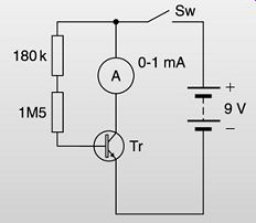
Fig. 1
Transistor testing
By comparison, the metal oxide semiconductor field-effect transistor (MOSFET) is fabricated around a current-carrying channel connected between the source and drain electrodes. Control of the unipolar current flow (meaning that it consists of either electrons or holes only) is obtained by way of a capacitive effect between a gate electrode and the base substrate. Modern MOSFETs have protection diodes incorporated, so that it’s possible to make meter readings that provide some indications of the condition of the MOSFET. This is not applicable to a MOSFET integrated circuit (IC), however. The simplest test is to switch the multimeter to the diode testing range and clip the negative lead to the MOSFET source and the positive to the drain. This should read an infinite resistance, no current passing. Placing the positive lead now on to the gate and then switching it back to the drain should show conductivity (because the gate retains the charge), and discharging the gate (one finger on the source and another on the gate) will drain the charge and the source-drain resistance will again be infinite.
==
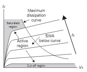
Fig. 2 Output characteristic for a BJT showing the various areas of operation
==
Causes of failure
Just as diodes can become open- or short-circuit, so similar faults can arise with BJTs between base and collector and base and emitter. Individual electrodes can become open-circuit and a condition known as punch-through can occur where a short-circuit develops between collector and emitter when the base region is ruptured, usually through excessive current and hence heat dissipation. Other faults that may be encountered are changes in input and output impedances and gain. In general, these are due to overdriving and the consequent dissipation of excessive heat.
For field-effect transistors (FETs) the insulation layer of silicon dioxide between the gate and substrate is the major weakness. The gate region is susceptible to damage through electrostatic discharges (ESDs) and, for this reason, this electrode is often protected by diodes built into the structure during fabrication to provide a shunt path for such discharges.
Fig. 2 shows the output characteristic for a BJT, and it’s also fairly representative of a power MOSFET. At a zero value of base current Ib, the collector current Ic is practically zero for all normal values of collector voltage, Vc. This is described as the cut-off region. As Ib and Vc increase so does Ic, as shown, and this represents the active region that is used for linear applications. At low values of Vc the collector current lies in the saturated region irrespective of the values for Ib. Since both saturation and cut-off regions represent areas of either practically zero voltage or current, the transistor dissipates very little heat and these are the regions used for digital operations. However, it’s important that the transition between on and off should be rapid to avoid generating heat and wasting power source energy.
This diagram also shows a maximum dissipation curve that describes the boundary of the safe working level of power [safe operating area (SOA) or safe working area (SWA) that the device can dissipate. It’s a curve drawn for all values of maximum power dissipation = Vc x Ic.
Semiconductor devices are relatively easy to test when out of circuit.
However, when included on a populated circuit board, the dynamic effect of any signals and the shunting effect of bias and other components give rise to misleading results.
Many modern digital voltmeters (DVMs) now include sockets for testing the gain (hfe) of small signal transistors. However, for other devices such as power transistors, although the basic circuit can be adapted it must be remembered that while small signal transistors usually have a gain that is measured in hundreds, the gain of larger power devices will be in the range of tens.
Dedicated transistor testers are available that can measure the parameters while the devices are in-circuit. In use, the circuit carrying the transistor to be tested is switched off, the test unit is connected to the transistor via short, low-resistance leads, and the residual effect of parallel circuit components is backed off with a balance control. Operating a push to test switch causes the meter to indicate the value of hfe. More sophisticated test instruments are available that can also measure the other important device parameters such as input and output impedances. Details of useful test instruments for semiconductors and other electronics components.
===
++++
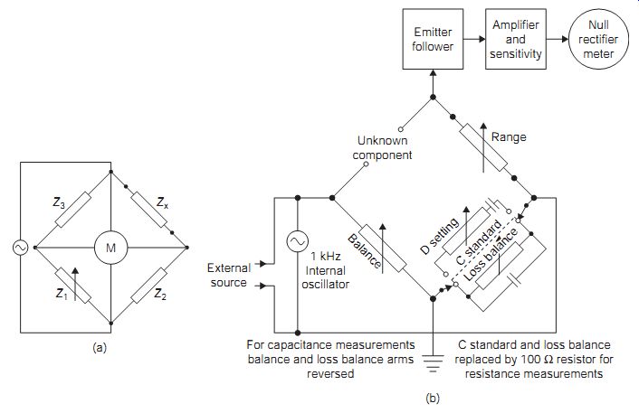
Fig. 3 Universal bridge [Marconi Instruments]
For capacitance measurements balance and loss balance arms reversed
C standard and loss balance replaced by 100 Ohm resistor for resistance measurements
Emitter follower Amplifier and sensitivity Null rectifier meter
External source 1 kHz Internal oscillator
===
+++
Experiment 2:
From a selection of BJT devices, some of which may be faulty, carry out forward and reverse resistance tests on the three termination pairs. Record the findings and compare the results with further tests carried out using a proprietary transistor tester.
+++
Using a universal bridge, compare the values obtained for a number of R, L and C components each with nominally the same values. In particular, inductors and capacitors can show a marked difference in loss values. It can also be useful to measure the self-inductance of some wire-wound resistors.
+++
Passive component testing
All discrete passive components suffer from ageing and heating effects and, since the latter are particularly cumulative, it’s important to avoid excessive temperatures during construction and repair. Furthermore, it’s important to avoid the hazards of solder fumes and the environmental effects of the lead content of solder. Typically, a tin/lead solder with a melting point of about 183ºC has been commonly used in the past, but this must now be replaced by lead-free alloys obtained from metals such as tin, copper, silver, indium and zinc. Like active devices, R, L, and C components are all more difficult to test in-circuit than as individual items. Hence, the simple solution is often to unsolder one end of the suspect device. All of these devices can be tested using a universal bridge tester.
Resistors very rarely develop low resistance values in use. They commonly go high in value or develop an open-circuit due to age or through passing excessive current and hence heat dissipation. Although front-line testing may usefully use a digital multimeter (DMM) switched to the ohms range, for the most accurate assessment of change of value, a Wheatstone bridge tester is by far the most effective.
Inductors (now less commonly used) may develop open-circuits through passing excessive current or simply by corrosion forming at the terminations. More commonly, inductors, like transformers, develop short-circuited turns which dissipate energy. This generates excessive heat and generally adds to the lossiness of the component. Even a short-circuit between two adjacent turns can lead to the faulty operation of any circuit to which the inductor is connected.
Capacitors are particularly sensitive to temperature effects and can develop into open- or short-circuits, change value or develop excessive leak age across the dielectric. Electrolytic capacitors are most susceptible to this problem. The important test for an electrolytic is the effective series resistance (ESR), which can be measured on an instrument similar to a DMM (ESR can even be included as one of the special DMM functions). In general, ESR is very low, usually less than 1 ohm, and represents the loss in phase angle between the current and applied voltage, which in theory should be 90º. Capacitors are commonly rated for operations at 85, 105 or 125ºC, so that if repeated failures occur, the replacement capacitor temperature rating can usefully be upgraded. Faulty capacitors, in general, are the most common source of circuit problems. The basic Wheatstone bridge circuit which was introduced to determine the values of unknown resistances can be extended to evaluate unknown inductors and capacitors. In this case, the bridge must be energized from an a.c. source, the unknown device must be compared with a similar standard component, and the null detector must include a suitable a.c. rectifier circuit.
The basic conditions for the bridge circuit at balance are that the products of opposite arms are equal. In the universal bridge, the product of the range and balance resistor values must be equal, at balance, to the product of the unknown impedance and the standard impedance.
The simple bridge can only determine the component value and not evaluate its losses. In general, it’s also necessary to determine the value of the equivalent series resistance of an inductor and the equivalent shunt resistance of a capacitor. In both cases, the resistive element represents the component losses which are related to its quality factor; the Q factor in the case of the inductor, and the loss angle (the angle by which the voltage/current relationship fails to reach the theoretical 90º) for the capacitor.
Figure 3 shows how the basic bridge concept can be adapted to provide universal features. This bridge circuit may be energized either from an internal 1 kHz oscillator or from an external source. Using an external 10 kHz source is particularly useful for measuring components with very low losses.
The null detector circuit and its amplifier and sensitivity control are buffered by an emitter-follower circuit to minimize loading on the bridge network. In application, the unknown component is connected into the appropriate arm of the bridge. The instrument is then set to measure an R, L or C component and a range is selected that provides a minimum meter deflection.
A lower minimum value is then obtained by adjustment of the balance control and this indicates the component value. By further adjustment of the loss balance control, a true zero meter indication can be achieved. The loss balance setting then indicates the resistive loss component. The range of measurements available with this instrument, with an accuracy of better than 1% of the reading obtained, is indicated here.
Certain of these instruments are designed for portable fieldwork and are therefore likely to be subjected to shock and vibration. Local service work is therefore likely to involve the repair of such ravages. Since the overall accuracy is critical, any repair work must be followed by recalibration. The necessary equipment for this is only likely to be found in specially set-up service departments.
Counter/timer
These devices, which range from simple handheld models to complex laboratory bench instruments, are chiefly used for measuring signal frequency (or pulse-repetition frequency) over a range, typically from d.c. to more than 2 GHz.
The operation is based on pulse-counting over a known period, from which the frequency is automatically determined. The readout is then commonly presented on a seven-segment liquid crystal display (LCD) or light-emitting diode (LED) display. The block diagram of the basic system, omitting the reset and synchronizing sections.
++++
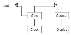
FIG. 4 Basic block diagram of a counter/timer: Gate Counter Display Clock
Input:
The counter section consists of a binary counter with as many stages as required for the maximum count value. The input to the counter is switched, and in the counting position, the input pulses operate the counter directly.
When the switch is set to the timing position, the input pulses are used to gate the clock pulses, and it’s the clock pulses that are counted.
Counter/timers are often microprocessor controlled with a basic clock frequency, typically of 1 MHz in older units and higher frequencies in modern units. This is provided either by a temperature-compensated crystal oscillator (TCXO) or by an oven-controlled crystal oscillator (OCXO). Provision is often made for two-channel (A and B) measurements and these inputs may have different upper cut-off frequencies. Low-frequency noise can be troublesome with these instruments and so a low-pass filter with a cut-off frequency at about 10 kHz is often used at the inputs.
Facilities include absolute frequency, phase, period and time measurements, with frequency and time ratios for the A/B channels. Selectable gate times are used to extend the range of measurement. To extend the frequency range even further, a pre-scaler (a frequency divider x10, x100) can be connected between the source and the counter/timer. Typical sensitivities range from about 20 mV at 5 Hz to about 150 mV at 150 MHz, with input impedances of the order of 1 M in parallel with 40 pF. As for the cathode-ray oscilloscope (CRO), x10 probes are usually available for use with signals of an amplitude greater than the in-built attenuator can handle. The resolution (the smallest change that can be registered) varies from about 0.1 Hz at the lower frequencies to 1 kHz at high frequency.
Microprocessor-controlled instruments allow for the inclusion of more elaborate features, such as hard-copy printouts and links to automated test equipment (ATE) networks.
Apart from power-supply problems, all the fault tracing will use digital techniques. Again, it’s important that any service work should be concluded by recalibration, therefore this form of work should only be entrusted to suitably equipped service departments.
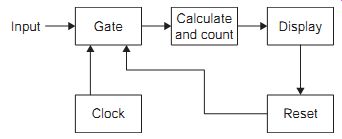
Fig. 5 Block diagram of a basic frequency counter: Gate Calculate and
count; Display; Clock Reset; Input
Frequency meter
The frequency meter makes use of a high-stability crystal-controlled oscillator to provide clock pulses. The instrument may either be combined with a counter/timer or provided as a function of a complex DMM, in which case, the accuracy will be somewhat reduced. In its simplest form, the unknown frequency is used to open a gate for the clock pulses.
The number of clock pulses passing through this gate in the period of one input cycle will provide a measure of the input frequency as a fraction of the clock rate. E.g., if the clock rate is 10 MHz and 25 cycles of the unknown frequency pass the gate, then the input frequency is 10/25 MHz, which is 400 kHz. A calculating and counter-circuit then passes this result to the display stage to give a direct indication of the input frequency.
In this simple form, the frequency meter cannot cope with input frequencies that are greater than the clock rate, or with input frequencies that would be irregular submultiples. For example, it cannot cope with 3.7 gated pulses in the time of a clock cycle. Both of these problems can be solved by more advanced designs.
The problem of high frequencies can be resolved by using a switch for the master frequencies that allows harmonics of the crystal oscillator to be used. The problem of difficult multiples can be solved by counting both the master clock pulses and the input pulses, and operating the gate only when an input pulse and a clock pulse coincide. The frequency can then be found using the ratio of the number of clock pulses to the number of input pulses.
Suppose that the gate opened for seven input pulses and in this time passed 24 clock pulses at 10 MHz. The unknown frequency is then 10 _ 7/24 MHz, which is 2.9166 MHz. Frequency meters can be as precise as their master clock, so that the crystal control of the master oscillator determines the precision of measurements.
The instrument is useful for checking and adjusting a wide range of oscillator settings, crystal oscillators in frequency conversion stages, display driver clocks and motor speed controllers.
The readout should extend to at least eight and preferably 10 digits, with an accuracy of at least 2 ppm (parts per million: 2 in 10^6 ) and a sensitivity of at least 10 mV. A pre-scaler can be used to extend the range of frequency operation, and pre-selectable gate times of 0.1, 1 and 10 s are often provided, but with progressively longer settling times.
For recalibration purposes, a service accessible preset adjustment provides a means of checking the master oscillator setting against some frequency standard. In the absence of a suitable laboratory standard use can be made of the 50 Hz and 15.625 kHz field and line frequencies from a television receiver, the broadcast colour television subcarrier at 4.43361875 MHz or even the BBC long-wave program at 198 kHz, whose carrier is maintained to an international frequency standard.
===
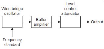
Fig. 6 Block diagram of a low-frequency signal generator: Wien bridge
oscillator Frequency standard Buffer amplifier control attenuator; Output
===
Low-frequency signal generator
Some equipment cannot be tested without an input signal. Very often a signal generator will make measurements easier than the sensor or system that is used in actual operation. Applying a single frequency at controlled amplitude to an audio amplifier, allows measurement of gain, and changing the frequency can explore the bandwidth.
By comparison with other signal sources, these instruments are relatively simple devices, but if they are to be trusted they must be well designed and constructed. As shown, the fundamental frequency is generated typically by a Wien bridge oscillator stage because of its wide basic frequency span. This stage is followed by a buffer amplifier to isolate the oscillator from the effects of any load. The output signal level is controlled by an attenuator stage that delivers an output typically at 600 Ohm impedance.
Low-frequency signal generators are usually used for the setting up and servicing of audio systems and as such they produce output signals of both sine- and square-wave form. The frequency range usually covers from 10 Hz to 1 MHz in five switched decade bands, with a frequency accuracy ranging from 1% to 5% at full scale.
Because of the needs of hi-fi systems, these generators usually provide a very low level of sine-wave distortion, typically better than 0.05% over the range 500 Hz to 50 kHz. Off-load outputs of 20 V peak-to-peak (p-p) are common, with the level being controlled in a series of steps of x10 or x20 dB, down to about 200 mV minimum.
=====
Experiment 4
Measure the stage gains of a three-stage audio amplifier using the controlled output of a low-frequency signal generator, together with a suitable instrument to measure the signal amplitudes. Evaluate the -3 dB cut-off frequencies to determine the bandwidth for the complete amplifier.
====
Function generators
Basically, these are signal generators designed to produce sine, square or triangular waves as outputs. Each may be varied typically over a frequency range covering from less than 1 Hz to about 20 MHz. The basic frequency may be generated either by a highly stable oscillator circuit, or by using a frequency synthesizer. The output levels are typically variable between about 5 mV and 20 V peak of either polarity, plus a transistor-transistor logic (TTL)-compatible signal at 5 V. Some of the basic waveforms. The output impedance is nominally 600R and provision is made for driving signals via balanced or unbalanced lines.
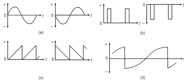
Fig. 7. Function generator waveforms: (a) sinusoidal, (b) positive and
negative pulses, (c) positive and negative sawtooths (serrasoids), and
(d) compound wave
Each of the basic output signals is capable of being modified. The sine wave may often be phase-shifted, and the square wave mark-to-space ratio is variable so that a pulse stream of variable-duty cycles can be provided.
The triangular wave can be varied to provide a sawtooth of varying rise and fall periods. In addition, it’s also possible to add a d.c. value to each output as an offset. This is valuable for testing circuits that are d.c. coupled and with a frequency response that extends down to zero. The square wave is also differentiated and integrated to generate exponential envelopes (see the block diagram).
===
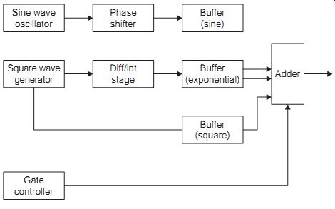
Fig. 8 Block diagram of function generator: Buffer (exponential); Buffer
(square); Adder Diff/int stage; Square wave generator; Gate controller;
Buffer (sine); Phase shifter; Sine wave; oscillator
===
An additional feature often allows a second signal component to be gated into the primary waveform, as indicated. A further variation of this is the tone burst that consists of a sine wave modulated with a parabolic envelope, but generated in bursts. This waveform is particularly suited to the testing of full-bandwidth audio systems or those circuits where strange resonances may occur. A variation of this feature uses a form of frequency modulation (FM). Here, a basic sinusoid is frequency-swept between predetermined limits, at either a linear or a logarithmic rate.
The more sophisticated instruments in this range may be equipped for microprocessor control, and have a digital readout of frequency and amplitude, plus a built-in standard frequency source.
It’s most important that the instrument calibration is carefully checked following any repairs. Service work is therefore a very specialized operation.
Integrated circuits are extensively used, together with stabilized switched mode power supplies. The highly critical oscillator circuit is invariably temperature controlled.
Decibel measurements
Measurements of gain or loss scaled in decibels can be made using an intelligent DMM. An intelligent DMM allows for automatic selection of ranges and for true root mean square (r.m.s.) measurements, so that amplitude measurements can be made. Measurements of power loss and gain can be carried out with such an instrument, and some can also measure signal-to noise ratios.
PCs and iPads as test instruments
With the introduction of the personal computer (PC) to the workshop environment, initially for information only, a wide range of hardware devices that are software controlled became available. These range from fairly simple and low-cost active probes capable of providing the actions of storage oscilloscope, spectrum analyzer, DVM and even transient recorder functions, through DMM, storage scope with spectrum analyzer, transient recorder, plus function generator, to high-cost extensive networked systems that provide all of the above, plus remote data logging from test benches, etc.
In general, these all have one point in common: they are attached to the PC via the parallel printer port, a specially provided plug in parallel port card or, more recently, the universal serial bus (USB) connector. For oscilloscope simulation the sampling rate of analog-to-digital conversion (in MS/s) must be at least twice the bandwidth for sine waves and preferably higher (up to eight times the bandwidth) for a complex signal.
Although there are other suppliers of virtual instrument (VI) equipment, the following devices and systems that run in the familiar Windows environment, with typical task bars and pull-down menus, have been extensively evaluated for the servicing environment. These are manufactured by:
• National Instruments (ni.com)
• Fluke
Of the three manufacturers, National Instruments (NI) probably provides the most extensive range of measurement, data acquisition (DAQ), data logging including image acquisition, and signal conditioning accessories for a system that is more likely to be used in a product life testing and monitoring environment. Since the system is designed to operate with real-time applications, in a measurement, control and statistical analysis mode, it’s capable of being coupled into a wide range of communications networks that include back-plane bus extensions, Internet, general-purpose interface bus (GPIB), Ethernet, fire-wire (IEEE1394) and USB.
Standard function generator waveforms including composite video are provided, plus many more that are user programmable. These offer:
• sine and square waveforms at frequencies up to 105 MHz
• linear and logarithmic frequency sweeps and bursts
• multi-device synchronization for channel expansion
• frequency resolution up to 1.07 µHz using direct digital synthesis.
The DMMs have 5.5 digit accuracy for a.c. voltage and current (true r.m.s.), d.c. voltage and current, and resistance. These are used to measure the outputs from many different types of transducer on several channels virtually simultaneously.
The data-capture analog-to-digital converters (ADCs) or digitizers can be driven from a wide range of transducers via appropriate signal conditioners, ranging from resistance temperature detectors (RTDs) to thermocouples, thermistors, chromatography sensors, strain gauges, force, load and pressure sensors, and linear displacement devices such as the linear variable differential transformer (LVDT). Bandwidths vary from 100 MHz down to 4 MHz, while the corresponding resolution ranges from 8 bits up to 21 bits.
Because of the complex nature of the NI system, the manufacturer provides extensive technical backup comprising system development support, technical training and future development. The website also offers training videos online, which are very useful in deciding how to make use of the products. For lower level servicing applications, however, the NI equipment may be seen as over the top for a small workshop.
++++
Experiment 5
The waveform shown can be used to derive the relationship between the peak and r.m.s. value for a symmetrical square wave as follows. Squaring the voltage waveform that swings between -0.4 and +0.4 V produces a new wave for V2 as follows: (-0.4)2= +0.16 and (+0.4)2 = +0.16
Practical:
The average value for V2 is thus 0.16 and continuously positive. Taking the square root of V2 produces the values of 0.4 V, again continuously positive. Thus, for the symmetrical square wave the peak and r.m.s. values are equal. This is only true for square waves; all other shapes have a variation in this relationship. Now suppose that the addition of a d.c. offset produces an asymmetrical square waveform that swings between -0.2 and +.6 V (amplitude is unchanged). Repeat this exercise and compare the results.
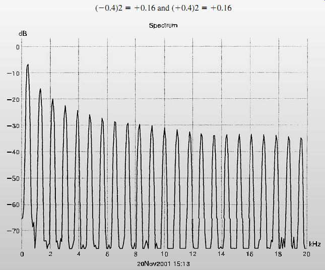
Fig. 9 CRO display of square wave signal in time domain.
++++
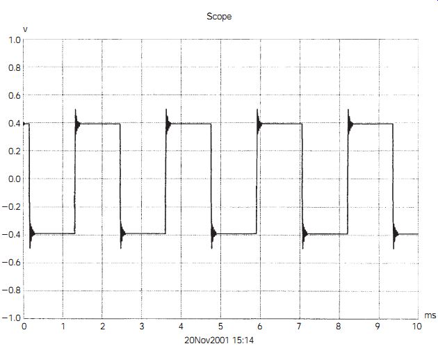
Fig. 10 CRO display of square wave in frequency domain.
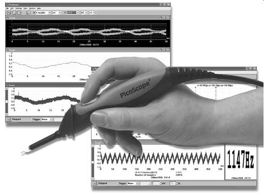
Fig. 11 Fluke handheld oscilloscope
The Fluke system provides similar types of function, but with lower accuracy and less sophistication and at lower cost than the NI system. This is an economical alternative to standard test equipment and data acquisition tools.
The system software and documentation are supplied in the most European and Asian languages (or use Google translate), with a backup service via the Internet and website. The system is fully developed to CE under ISO9001 standards. It functions on most of the early PC developments from DOS software and 80386 or higher processors supported by downloadable updates from the website. Some adapters plug into the PC parallel, others into the USB connector, and the power supply of an adapter is taken from the port; no separate supply is needed.
In the time domain, the main screen of the oscilloscope provides for both normal timebase and X-Y operations. The latter is particularly useful when comparing two time-related waveforms such as found with advanced modulation schemes. The spectrum analyzer provides an alternative view of a signal in the frequency domain. Switchable probes of 110 or 10/100 are available, in either 60 MHz or 250 MHz form.
In the digital storage CRO mode, the sampling speeds depend on the model that has been selected. Fluke offers oscilloscope adapters in ranges described, as simple, general-purpose and high-speed, with sampling rates ranging from 20 to 200 MS/s, with comparable analog bandwidths. Both waveforms and instrument settings can be stored on disk for future study and analysis.
When equipped with suitable sensors/transducers, the data acquisition and logging software can measure temperature, humidity, sound pressure, light, current, resistance, power, speed and vibration levels. This data can be transferred to other Windows applications over local area networks or the Internet using the copy and paste facility. The data can also be displayed in a spreadsheet format, such as Excel, with analysis of data trends.
The Fluke handheld oscilloscope is particularly suitable for field service (used along with a laptop computer). The large probe is plugged into a USB port, needing no other source of power, and requires no additional connections or installation procedures. The design allows for single-handed operation, with control accomplished by a button which is pressed to start the oscilloscope action and which flashes green to indicate that the oscilloscope is active. The tip of the probe is illuminated to make it easier to locate the point at which the signal is to be examined. When the signal has been captured on the computer screen the button can be pressed again to stop oscilloscope action: the button then glows red. If the button is held down it will activate the auto-setup action to configure timebase and triggering.
The supplied software will provide oscilloscope, spectrum analyzer and metering functions, and additional software can be bought to add data acquisition.
+++
Experiment 6:
With a PC virtual instrument, connect the system to a working three stage low-frequency amplifier to measure the frequency response, bandwidth and gain of the individual stages. Using the spectrum analyzer and an input from the function generator set to 100 Hz sine and square waves, note the change in the harmonic content at the amplifier output.
+++
Servicing information:
With the introduction of computing systems, the lifetime of the hard-copy service manual is nearly over. Much of today's service information is now provided either on CD-ROM or via the Internet. In earlier times, the service technician's manual carried not only the original service diagram and data, but also a lot of personal information that he or she had gleaned over time about that particular system. Trying to read today's manual from a monitor screen is certainly a different experience. Following the diagram of such as a television receiver, with interactions across many screens, appears at first sight virtually an impossibility. Even printing out sections of the diagram and gluing them together with sticky tape is not conducive to best use of the servicing bench. Fortunately, most electronic-based service information provides space in memory for the technician to add further comments as aids for future use. However the service information is provided, via the web, CD, YouTube, DVD or even satellite links, new skills will have to be developed to make the most of what could be information overload.
Technicians servicing domestic electronic equipment are generally well provided with circuit diagrams and data sheets, but to produce a thoroughly reliable and economical repair that will generate customer loyalty, they need additional skills and support. Not only is it necessary to understand how the system works, there is also a need to have a knowledge of the system's historical reliability and its particular points of failure. In the past, when systems were constructed largely from discrete components, many of the failures occurred in a regular manner, giving rise to the stock faults.
Indeed, many service departments found these to be a source of good business that created a sound reputation for doing a good job.
With today's extensive use of dedicated ICs the system reliability has improved considerably. However, stock faults still occur, but repeat very much less frequently, making a good memory an additional requirement for service personnel. One of the best service aids is a subscription to the journal Television (see below). This acts as a clearing house for the hints, tips and solutions to problems encountered by many practicing service technicians. Fortunately, there are now a number of computer system databases available that have been designed to aid the servicing of such equipment.
While these can provide almost instant access to many of the stock faults, it must be emphasized that these should be used in conjunction with the manufacturer's circuit diagrams and data sheets.
The website (www.servicemanuals.com) extremely useful for servicing information that is hard to get or out of print, and for anyone in a hurry, a manual can be downloaded for almost immediate access.
Of these databases, two have been tested and found to be invaluable to the busy workshop.
The first one tested was formerly provided on CD-ROM and is now available from the magazine publisher. THIS publishes, among others, the magazines Electronics World and Television and Electronics Online. The fault-finding and repair hints represent the knowledge gleaned from manufacturers, dealers and repair centers, and cover about 1 million entries from more than 400 manufacturers. Unusually, the database information is covered in most European languages. Originally, information was sent out on CD-ROM, but this has now been superseded by a completely online ser vice, for which you need to register to obtain servicing tips (although lists of stock faults can be seen without registration). The requirements for your PC are:
• Windows PC, Linux and Apple
• 32-bit operating system (Microsoft Windows XP or higher, Apple OS)
• graphics card high color or higher
• resolution 800 x 600 or higher
• browser: Microsoft or Netscape version 4.01 or higher
• Java Script active
• cookies allowed
• Java Engine installed and active.
Some other useful servicing-related websites for technical data, service sheets, spares and data are listed at the end of this section.
+++
Experiment 7
Compare information from several different sources in relation to a fault condition.
+++
QUIZ:
1. The safe operating area (SOA) for a
transistor is located:
(a) at the lowest possible value of bias
(b) when the transistor is nearly
saturated
(c) between the cut-off and saturation
points
(d) when the current is a maximum.
2. All types of passive components can be
tested using:
(a) a multimeter
(b) a bridge type of circuit
(c) an oscilloscope
(d) an ohmmeter.
3. You would use a counter/timer typically for:
(a) measuring the time a task took
(b) measuring the frequency of an oscillator
(c) measuring the number of times a fault occurred
(d) measuring the mean time before failure.
4. An LF generator will probably use:
(a) an LC circuit
(b) a shift register
(c) a Schmitt trigger
(d) a Wien bridge circuit.
5. An advantage of using virtual instruments is:
(a) they can make use of a spare computer
(b) they are more precise
(c) they can record readings as well as measuring them
(d) they make use of software.
6. The main advantage of getting servicing information from the Internet is that:
(a) it’s more accurate
(b) it’s more up to date
(c) it’s faster and requires no storage
(d) it’s better illustrated.