(source: Electronics World, Aug. 1964)

By J. RICHARD JOHNSON
Technique of using secondary standard, checked against WWV, to measure transmitter or r.f. generator frequency. Simple equipment can be employed to obtain accuracies far beyond that needed for FCC frequency requirements.
WHATEVER portion of the broad field of electronics holds your interest, frequency and frequency measurement are undoubtedly important to you. They are important not only to the performance of your equipment, but often, as in the case of transmitters, are factors which must be considered to avoid violations of the law.
Almost anyone with a basic knowledge of electronics, a modest amount of equipment, and the requisite care and patience can utilize the standard frequency broadcasts from National Bureau of Standards stations like WWV. Under such conditions, measurements accurate to within 1 part per million, or equivalent to an error of only one second in almost two weeks, are not unusual.
This article covers the use of a secondary frequency standard, checked against WWV, to make frequency measurements in the range between 1 mc. and at least 30 mc. A complete frequency-measuring system of this type is illustrated in block diagram form in Fig. 1.
One of the advantages of this type of frequency measurement is that a high degree of precision can be realized from relatively low-cost equipment. All you need is a reasonably good communications receiver, a 1000 /100 kc. frequency standard (often a TV marker generator will do), and a calibrated audio oscillator. With these and a little care, you can achieve accuracy far beyond that needed for even the most rigorous of FCC frequency requirements.
Direct Frequency Determination
If the frequency is very low, the most obvious method of measuring it is to count the cycles as they occur and then to determine how many cycles there are during a second, an hour, a day, or during any other specified period of time.
A simple example is the rotation of the earth. By definition, the rotational frequency is 1 cycle (revolution) per clay. Using the sun or some star as a reference, we can "count days" as the earth spins on its axis. Since a day is defined as 24 hours, we can express the earth's rotational frequency in different units: 1 cycle per day; 1/24= 0.0417 cycle per hour; 0.0417/60= 0.000695 cycle per minute; and 365 cycles per year. This example is more than just a random one, because the "mean solar day" is an international standard for the unit of time.
As the frequency increases, the human counting method not only becomes less accurate, but also fails completely when the cycles come so fast that the operator can no longer distinguish individual cycles. This usually happens at about 0.5 to 10 cps.
Cycle-counting can be done electronically at moderately high frequencies, but the human direct-counting method can be used only in very special applications in which the frequency is very low and human errors in timing can be tolerated, or in which the measured signal is recorded with a time base.
In all practical frequency-measuring techniques, signals of unknown frequency are compared with other signals whose frequencies are accurately known. This comparison is made practicable by the use of heterodyning.
Principles of Heterodyning
When two alternating currents of different frequencies f1 and f2 flow together in a non-linear mixer circuit, they generate a series of additional signals whose frequencies are equal to f1 + f2, f1- f2, f1 2f2, f1- 2f2, f1 + 3f2, f1- 3f2, etc. The first-order signals, at f1 + f2 and f1- f2, are of primary interest here. These are often referred to as the sum and difference heterodynes. These heterodynes are not generated unless the mixer circuit has a non-linear impedance. This non-linear impedance can be supplied by a vacuum tube, transistor, or solid-state diode, providing it operates over the non-linear portion of its characteristics. Thus one cannot hear a heterodyne signal from two r.f. signals applied to a pair of linear-impedance headphones even though the frequencies of the two signals differ only by an audio frequency. The two signals must be applied to a diode or other mixing device.
Fortunately, there is such a mixing circuit in any superheterodyne receiver ( and therefore in almost any receiver now in general use), i.e., the second detector circuit. Therefore, when we want to heterodyne r.f. signals to accomplish frequency measurements, we often need only apply them to the antenna terminals of the receiver and the low-frequency heterodyne signals can be heard at the receiver's output. This is the kind of process that takes place when a.c.w. signal is received on a communications receiver. The beat oscillator associated with the receiver's detector circuit heterodynes with the received signal (after conversion to intermediate frequency) and the heterodyne is the tone by which it is "copied." Suppose two signals of frequencies f1 and f2 respectively are heterodyned to produce a difference beat (heterodyne) in the audio-frequency range. Suppose further that f1 is to be measured and f2 is accurately known. Frequency f1 can then be determined by careful measurement of f1- f2 and addition of this frequency to f2. Because a difference heterodyne is often easier to measure precisely than the unknown frequency, the difference-heterodyne method is the one most often used in high-precision measurements. In such measurements, f2 in the above example is a frequency standard that has been either provided directly by the National Bureau of Standards standard-frequency broadcasts or by standards that have been checked against them.
Secondary Frequency Standards
Because of the complicated equipment required, astronomically checked primary standards are maintained at only a few locations. (Refer to the article "Frequency and Time Standards" in this issue.) However, this is not a serious handicap, thanks to the standard time and frequency broadcasts made available by NBS in this country and by government agencies in some other countries.
Our own NBS broadcasts provide a wide variety of standard time and frequency signals of extreme accuracy. The most important in the applications we are now considering are the reference standards provided by the carrier frequencies of these stations. These frequencies, as transmitted by WWV, are kept accurate to better than 1 part in a hundred billion or one ten-thousandth of a cycle per second at 10 mc. (outside of a fixed frequency offset of-1.50 parts in 10^10). Accuracy at the receiver is on the order of 1 cps at 10 mc. (0.00001 %) due to ionosphere instability. With the lower frequency stations, WWVB and WWVL, accuracy at the receiver is much better. The frequencies and types of transmission from NBS stations are given in Table 1.
Frequency measurements of great accuracy can be made at any location within range of the standard broadcasts by employing a .secondary frequency standard which is itself quite stable and whose accuracy can be optimized by alignment with the transmissions from the NBS broadcasts.
The simplest type of secondary frequency standard is illustrated in block form in Fig. 2. It is a stable crystal-controlled 100-kc. oscillator. The oscillator is equipped with a trimmer capacitor connected across the crystal, or with some other arrangement to allow very small adjustments (up to several hundred cycles per second) of the frequency of the generated signal. This allows compensation for variations in the oscillator frequency due to such things as temperature and voltage variations. A typical 100-kc. crystal oscillator circuit suitable for use as a secondary frequency standard is shown in Fig. 3.

Fig. 1. Complete, accurate frequency-measuring system.

Fig. 2. Arrangement of the simplest secondary standard.
The oscillator output contains not only the 100-kc. fundamental signal, but also harmonics at integral multiples of 100 kc. throughout the useful frequency range. One of these harmonics ( say the 50th, at 5 mc.) is tuned in on a receiver that is also receiving a standard broadcast from WWV on that frequency. The two signals beat or heterodyne, producing a third signal having a frequency equal to the difference between the frequencies of the local standard and the standard broadcast. Calibration checks of the secondary standard are made by adjusting the trimmer on the oscillator until there is zero beat between the oscillator harmonic and the WWV signal. When the oscillator frequency is very close to that of WWV, a slow pulsing (beating), indicating a difference heterodyne on the order of 1 or 2 cycles per second, can be heard in the earphones or loudspeaker or seen as fluctuations of the pointer on the receiver's "S" meter.
Much of the time WWV transmits tone modulation at either 440 cps or 600 cps (as well as pulse-type second markers) . It is preferable not to make secondary standard zero-beat adjustments while the tone is on. The audio frequency beat between the signal from the frequency standard and WWV's carrier, in turn, beats against the tone modulation signal, giving a false zero-beat indication. For example, suppose WWV is sending a 600-cps tone. If the harmonic of the signal from the standard is 0.6 kc. higher or lower in frequency than 5 mc., a 600-cps beat tone is produced and beats against the 600-cps tone modulation, causing an effect very much like that when the r.f. signals themselves are zero-beat.
Fortunately, it isn't necessary to make the adjustment while the tone is on. Starting at 3 minutes after the beginning of each 5minute interval, there is a period of almost 2 minutes when the tone and all other modulation except the second markers are off and thus the difficulties just mentioned are avoided. The details of the typical WWW modulation during each 5minute period are shown in Fig. 4. The one exception is the 5minute period starting at 45 minutes after the hour, when WWV goes off the air entirely for a period of 4 minutes.
Although a 1-cps or lower beat can normally be obtained, even with modest equipment, between the secondary standard and WWV, let us be conservative and assume maintenance of the oscillator frequency only to within 5 cps of that of WWV, so that the frequency error is limited to 5 cps in 5,000, 000 cps or 0.0001 %. Since the harmonics of the 100-kc. oscillator are all exact multiples of the fundamental oscillator frequency, they are all accurate to within the same percentage. Thus, any harmonics, in any part of the frequency spectrum, can be used as frequency markers for reference in making measurements.
Often a communications receiver is equipped with a crystal-controlled "marker" oscillator, whose harmonics are used to check the receiver's dial calibration. Such an oscillator is excellent for moderately accurate checks at 100-kc. intervals and can, like the frequency standard, be synchronized to WWV if equipped with a trimmer.
For example, if a measurement were to be made of some frequency near 20 mc., there would be frequency markers at 19.8, 19.9, 20.0, 20.1, 20.2, etc., mc. If the receiver has an accurately calibrated dial, these markers can be used as checks of receiver calibration so that rough readings of frequencies between can be made right from the receiver's dial.
For a heterodyne frequency meter whose output is also fed into the receiver, the 100-kc. harmonics can provide accurate calibration references.

Fig. 3. Typical circuit of oscillator useful as a standard.

Fig. 4. Type of information transmitted by station WWV.

Fig. 5. System that employs frequency standard with divider.

Fig. 6. Illustration of how signal at 15,019.1 is measured.
If the frequency to be measured falls close to one of the harmonics of the 100-kc. standard, it can be measured with great accuracy by measuring the audio frequency heterodyne between it and the harmonic. This is the process of interpolation and will be described in detail later. But if the frequency to be measured is spaced relatively far from either of the two adjacent harmonics, such precise measurement cannot be made. To provide the same accuracy at all frequencies, a frequency divider is added to the secondary frequency standard.
Frequency Divider
A properly designed multivibrator circuit can take an input signal with frequency f and put out a signal with a frequency which is some sub-multiple of f. In frequency standards, a multivibrator which divides by 10 is the most common. Fig. 5 shows how it is used to divide the 100-kc. frequency down to 10 kc. The 10-kc. signal, plus its harmonics, provides signals at 10-kc. intervals throughout the radiofrequency spectrum ( usually as high as to 100 mc. ) . Because the multivibrator divider is locked to the 100-kc. oscillator frequency, the frequencies of all these harmonics are equally accurate.
Consider the example of Fig. 6. As in the previous discussion, the 100-kc. oscillator of the standard is adjusted to within 5 cps of WWV on 5 mc., or within (5 / 5 x 10^6 )100- 0.0001% or 1 part per million. A measurement is then to be made near 15 mc. (say, on a frequency of 15,019.1 kc.) . Since 15 mc. is three times 5 mc., the adjustment tolerance, reflected in the 15-mc. signal is three times 5 cps, or 15 cps, which is still 0.0001% of the new 15-me. frequency. This accuracy now applies to all the 10-kc. harmonics, including those in the vicinity of 15 mc.
A typical multivibrator divider circuit for dividing from 100 kc. to 10 kc. is shown in Fig. 7. Frequency dividing is also sometimes clone by means of digital logic circuits, such as adders. These are used primarily where other associated circuits are of the digital type, but are usually not as practical as multivibrators in the majority of installations.
Interpolation
With a harmonic of precisely known frequency every 10 kc. through the spectrum, we have only 10 kc. between any pair to be covered. Thus no unknown frequency to be measured can ever be more than 5 kc. away from one of these harmonics. By heterodyning the measured signal against either the next higher or next lower 10-kc. harmonic, one can always come up with a beat signal in the audio frequency range.
Assuming that we can identify the 10-kc. harmonic we are using, we can simply add or subtract the frequency of the beat signal, depending on whether the unknown is above or below the nearest 10-kc. harmonic.
Consider the case mentioned earlier, in which the frequency to be measured is 15,019.1 kc. Before measurement, of course, this frequency is not known. However, the measured signal is found with the receiver dial between the 10-kc. harmonics at 15,010 and 15,020 respectively. By tuning from the unknown signal toward the 15,020-kc. harmonic we hear a beat note of lower pitch than in the other direction, so we know that the unknown frequency is closer to 15,020 kc. than it is to 15,010. The receiver is then tuned to give the strongest and clearest output of this lower beat signal.
Next, the beat signal is in turn measured by comparing it with a calibrated source of audio-frequency signal until the two audio-frequency signals are themselves at zero beat. If the beat signal is measured as 900 cps, it means that the unknown is 900 cps, or 0.9 kc. below 15,020 kc. and this places it at 15,019.1 kc. If the a.f. source is even moderately accurate, at least one more decimal place can be obtained. For example, if the beat signal is measured as 955 cps, the radio frequency is 15,020 minus 0.955, or 15,019.045 kc. If we should tune the receiver toward the 15,010-kc. harmonic, we would hear a beat signal of 10 kc. minus 0.955 kc., or 904.5 cps, which, being so much higher than the 955-cps beat, is not as easy to measure accurately.
The above process of determining the exact location of the unknown frequency in the spectrum space between known frequency-standard harmonics is called interpolation. The audio-frequency signal generator used to determine the beat frequency is referred to as an interpolation oscillator.
Interpolation Oscillators
An interpolation oscillator, in its simplest form, is a stable and accurately calibrated audio-frequency signal generator.
Any a.f. signal generator is suitable providing its calibration is accurate and stable enough. When using the interpolation oscillator, the accuracy of the over-all radiofrequency measurement depends on the accuracy of the a.f. calibration and on how high a radio frequency is being measured. For example, if the measured radio frequency is 50 mc., an a.f. beat signal accuracy of 100 cps is only 0.0002% of the radio frequency. A relatively inexpensive a.f. oscillator can read frequencies to within 100 cps, especially if below 2000 cps. On the other hand, at a measured frequency near 1 m.c., the interpolation oscillator must read accurately to 2 cps for the same relative r.f. accuracy.
Elaborate commercial interpolation oscillators are used in sophisticated frequency-measurement equipment. Accuracies are normally ±2 cps or better. The mixing circuit is usually self-contained. This is a circuit in which the a.f. beat between the unknown signal and the harmonic from the frequency standard can be mixed with the interpolation oscillator signal.
As in the calibration of the r.f. standard against WWV, the beat signal is heard in earphones or loudspeaker or by indication on an output meter.
Another popular method of comparing the interpolation oscillator frequency with that of the a.f. beat from the measured signal is through use of an oscilloscope and Lissajous figures.
This method is illustrated in Fig. 8. One advantage is that the interpolation oscillator does not need to be at zero beat, but can be set at some integral multiple or sub-multiple of the frequency that is being measured.
Use of 1-Mc. & Higher Markers
The procedure just outlined works well with just a 100-kc. reference oscillator and 10:1 divider at frequencies of approximately 5 mc. and below. But as the measured frequency gets higher, it gets more and more difficult to identify harmonics.
The 100-kc. harmonics can be distinguished from the 10-kc. harmonics by use of a switch that allows the divider circuit in the standard to be shut off, leaving just the 100-kc. signals.
However, at relatively high frequencies, the 100-kc. harmonics themselves bunch together so closely that, on most receiver dials, it is almost impossible to determine which one is which.
This problem is solved by adding to the frequency standard a 1-mc. crystal oscillator to help the operator, in effect, "get his bearings." With the 100-kc. oscillator turned off and the 1-mc. oscillator turned on, harmonics are found every 1 mc. throughout the frequency spectrum. The 1-mc. harmonic nearest to the measured frequency can be tuned in, then the 100-kc. oscillator turned on and the 100-kc. harmonics counted as the receiver is tuned away from the identified 1-mc. point. When the 100-kc. harmonic of interest has been identified, operation of the 10-kc. divider can be restored and 10-kc. harmonics counted, starting at the 100-kc. harmonic.
At frequencies above 20 mc., even the 1-mc. harmonics may not be sufficient to allow easy identification and some frequency standards also contain 5-mc. and /or 10-mc. oscillators.
These oscillators do not have to be referenced exactly to WWV, because the final measurement is with reference to the 100-kc. oscillator and its divided 10-kc. harmonics.
All the components of a complete frequency standard and interpolation setup are included in the block diagram of Fig. 1. With reasonable care and skill on the part of the operator, such equipment will permit measurement to within 5 cps on frequencies between 1 mc. and 5 mc. All of the components required are of the type whose nature and use has been discussed in this article.

Fig. 7. Typical multivibrator for dividing from 100 kc to 10 kc.
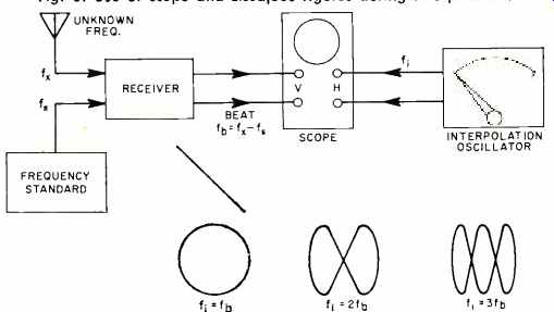
Fig. 8 Use of scope and Lissajous figures during interpolation.

Table 1. Information about standard broadcasts by NBS stations.