(source: Electronics World, Mar. 1966)
By JAMES F. KENNEDY
Once you know how a square wave is made up, this useful waveform can be used to rapidly test an over-all system.
SQUARE waves are not only useful in testing audio amplifiers but they also occur in television, radar, digital computers, and many other types of modern electronic circuitry. For this reason, a knowledge of the makeup and use of square waves is vital to nearly everyone who deals with electronics.
With fifteen or twenty audio signal generators and lots of patience, a pretty good square wave could be developed.
First, select a fundamental frequency of, say, 100 Hz of sine wave at a convenient amplitude. Then mix that with the third harmonic of the fundamental, or 300 Hz of sine wave at one third the amplitude of the fundamental. From the next generator, feed in the fifth harmonic of the fundamental at one-fifth the amplitude; then the seventh harmonic at one-seventh the amplitude of the fundamental; and so on. Arrange it so all of these sine waves are exactly in phase (starting at the same time).
Fig. 1A shows how these waveforms will combine to form a square wave. As more and more odd harmonics having the proper phase and amplitude are added, the resultant wave form comes closer to a perfect square wave.
There are several important things to be learned from this analysis. First, a square wave is made up of a number of sine waves: it- consists of the fundamental and a great number of odd harmonics. The higher the harmonics go, the closer the final resultant waveform will resemble a square wave.
Second, notice from Fig. 1A that the fundamental and the lower harmonics fill in the flat top portion of the square wave.
Third, note that the higher harmonics contribute to the steepness of the leading and trailing edges of the waveform and to the squareness of the corners at the top.
If you feed a square wave into an audio amplifier and look at the result on a scope, you will actually be testing the amplifier from about one-tenth of the fundamental frequency up to about 40 times that frequency. The amplifier may handle a sine-wave input with no difficulty, but a square-wave test is much more realistic, as the amplifier is now being called on not only to handle the fundamental frequency, as it would do with a sine-wave input, but it is also being asked to amplify all the harmonic components in the wave equally, without changing the phase of any of them.
When a signal is passed through a capacitor, the voltage lags the current, and vice versa when the signal goes through an inductance. Most amplifiers use coupling capacitors. At medium and high frequencies, the reactance of the capacitors is negligible, but as the frequency goes down, the reactance increases until it may be considerable. When a capacitor is operated with a following grid resistor, for example, the combination will act like a frequency-sensitive voltage divider, reducing the level as the frequency goes down. Depending on the relative values of this pair of components, a certain amount of phase shift will also occur. This means that at the lower frequencies, the signal will be changed in phase and amplitude compared with a higher frequency signal. This is called phase distortion.
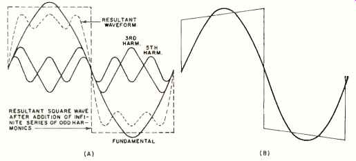
Fig. 1. (A) Adding a large number of odd harmonics to a sine wave produces
a square wave. (B) Phase lag of the fundamental.
Fig. 1B shows the effect on the shape of the waveform if the fundamental is delayed in phase. Since time is read from left to right on the diagram, a lag in the fundamental frequency means that it will be displaced to the right, as shown.
Note that the right-hand, or trailing, edge is higher in amplitude than the left-hand, or leading, edge. This is also called "tilt." If there is a phase lead, the lower frequency components will be moved over to the left and the tilt will be in the other direction.
This particular amplifier would put out a good sine wave at 20 Hz, and there would be no clue as to the phase distortion present if it were tested with just a sine-wave signal.
As previously mentioned, capacitive reactance increases as the frequency goes down. This means that the output of the amplifier will fall off at the lower frequencies. Because the lower frequency components of the square wave contribute mostly to the flat top of the waveform, if these components are made weaker, or attenuated, the flat top portion will sag, as shown in Fig. 2A. This illustration shows the results on the shape of the square wave if the fundamental or the lower harmonics are attenuated while going through the amplifier.
However, this attenuation is usually due to reactive components in the amplifier, that is, the effect of capacitance or inductance on the waveform. This means that usually there is going to be not only attenuation but also some phase shift along with it. The effect of phase shift at the lower frequencies is to cause a tilt in the flat top, and the attenuation at these lower frequencies causes a sag in the flat top, so that it is possible to see something like Fig. 2B.
Too much output at the lower frequencies, called low-frequency boost, will show up as a bulge in the flat top portion, as in Fig. 2C. Another point should be evident from the fore going discussion: an audio amplifier cannot be tested by feeding in a square wave at just one frequency. A 20-Hz square wave will test up to about 40 times the fundamental, or 800 Hz. Obviously, this tells us nothing about the way the amplifier handles higher frequencies, say up to 20,000 Hz or so. If we divide 20,000 by 40 we get 500 Hz as a convenient value for our second test frequency.
Conversely, the 500-Hz test will tell us very little about the low-frequency operation of the amplifier. We have to be careful in choosing the frequencies for testing, too. If a 10,000-Hz square wave is used, the amplifier will be checked to 400,000 Hz.
The higher frequency components of the square wave con tribute to the sharpness of the corners of the waveform and to the steepness of the rise of the wave. Fig. 2D shows a rounding of the upper corners caused by attenuation of the higher frequency harmonics in the square wave. This is called roll-off.
Note particularly that the leading edge and trailing edge are both rounded, which shows that the phase of the high-frequency harmonics has not been changed with respect to the other frequencies in the wave. If we had both high-frequency loss and the phase shift (and this could happen), the wave form would look like Fig. 2E.
It is also possible to have one type of distortion at one end of the spectrum and a different type at the other end. Wave form shapes like Fig. 2F would indicate phase shift at the low-frequency end and high-frequency loss at the other end.
Too much amplification at the higher frequencies can result in a waveform with leading-edge overshoot like that shown in Fig. 2G.
Another type of distortion which may appear is evidenced by oscillation across the top of the waveform as in Fig. 2H.
This is an indication that the amplifier is breaking into oscillation or ringing at some very high frequency.
There is nothing to prevent using the same technique for checking video amplifiers. The video amplifier in a television set should handle a range of frequencies from about 25 Hz to 4 MHz. If there is attenuation at the higher frequencies, fine details in the picture will not be clear.
Fig. 3 shows some of the nomenclature used in pulse measurements and discussions. Probably the most frequently used term is "rise time," which is just what the name implies: the time for the pulse to rise from 10% to 90% of its maximum value. In checking a computer, for example, part of the procedure would involve measurement of the clock pulse to make sure that the rise time was within certain limits. This time is usually measured in microseconds or nanoseconds. The vertical amplifier of the scope used would have to amplify the pulse without distortion so that an accurate measurement could be made. Such an amplifier would be flat within 3 dB from d.c. to 15 MHz, 30 MHz, or even higher.
So far only symmetrical square waves, that is, square waves in which the pulse-width time and the resting time are equal, have been discussed. A radar transmitter or a television set might involve square waves in which the pulse width is only a small part of the total time. For instance, the pulse width might be one microsecond, or 1,000,000 of a second, and the pulse might be repeating 5000 times a second. These are nonsymmetrical square waves. The 5000 figure would represent the "pulse-repetition rate," which is generally used in preference to the word frequency. This pulse occurs for one micro second, 5000 times a second, or 5000 microseconds out of each second. Since there are 1,000,000 microseconds second, the pulse is actually present only 0.005% of each second and the rest of the time the circuit is resting. This is called the duty cycle and is one reason why such huge amounts of power may be developed with radar transmitters. The transmitter is operating for only a very small portion of the total time so that it can withstand tremendous overloads and then cool off until the next pulse comes along.
Short pulses of this type have a very fast rise time, which means higher frequency harmonics in the waveform and the fact that the amplifiers must handle an upper frequency limit equal to the reciprocal of the pulse width. For a pulse of one microsecond width, the amplifier would have to go up to at least the reciprocal of this, which is 1/0.000001 or 1,000,000 Hz.
Some radar receivers have a bandwidth of 5 MHz or more to properly handle short pulses without distorting them. In the case previously mentioned, the lowest frequency the receiver would have to handle would be 5000 Hz, which is the pulse repetition rate. This is equivalent to the fundamental frequency. The upper frequency limit is fixed by the pulse width, and even though the pulse may occur just once a second, if it is one microsecond wide then the amplifier must handle frequencies up to at least 1 MHz.
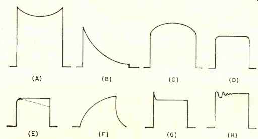
Fig. 2. Typical square-wave distortions. (A) Decrease in low frequency gain.
(B) Decrease in low-frequency gain plus phase shift. (C) Excessive low-frequency
gain. (D) Poor high-frequency response. (E) Poor high-frequency response plus
phase shift. (F) Low-frequency phase shift plus loss of high frequency gain.
(G) Excessive high-frequency response. (H) Oscillation occurring at a high
frequency. In all these wave forms, it is assumed that the oscilloscope is
not at fault.
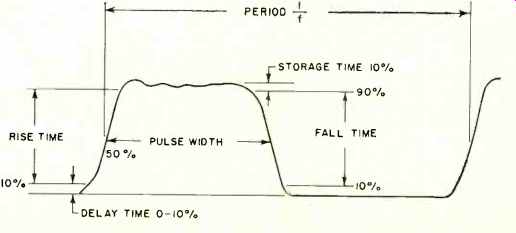
Fig. 3. Complete nomenclature for defining a square wave.