(source: Electronics World, Apr. 1968)
By WILLIAM M. STUTZ / Sr. Lab Technician, T.R.G. (Div. of Control Data Corp.)
The newer filters, such as Butterworth, Chebyshev, and elliptic types, are more accurate and easier to design.
WITH the many advances being made today in the field of semiconductors, it is almost impossible to keep abreast of developments. Therefore, it is not strange to find that familiar old passive circuits have advanced too. One particular area, filters, has changed radically from what many remember from technical school and college days. The old filters, such as constant-K and M-derived types, have been replaced by the Butterworth, Chebyshev, and elliptic types. These newer designs have much to recommend them. Their responses are more accurate over a wide range and are easier to design. (Fig. 1 ) The constant--K and M--derived types were traditionally designed section by section. This method was involved since each section had to be matched while trying to optimize the response. The results of such designs were approximate to say the least. Today the filter is designed as a whole, which simplifies the matching and allows us to optimize the response. Both problems actually reduce to almost "cookbook" simplicity in most cases. The third problem in filters, realization, now becomes the main problem.
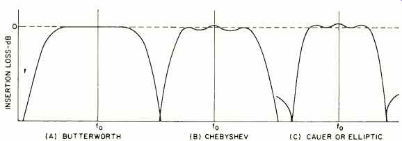
Fig. 1. Response curves of the three filters described in text.
The actual mathematics involved in a filter design today is very abstract and is usually best left to the mathematicians. The filter's properties are expressed by a transfer equation that is a function of frequency. The shape of the response is then set, but actually that is all that is permanent. The frequency and impedance information contained in such a transfer equation may be extracted. The remaining information is said to be "normalized ". A normalized number or quantity may then be used under a large number of circumstances as opposed to the unique value or quantity simply by supplying the missing information to de-normalize the quantity. This mathematical trick allows us to catalogue the elements of a specific filter type and to design from them a filter of any particular bandwidth or impedance value that we require.
Originally, the term "realization" meant the mathematical realization process. This requires at least a mathematician and at most a digital computer. The tern now means the physical as well as mathematical processes of determining the actual L and C component values to be used. I prefer the terms "de-normalization" and "realization" to distinguish the two.
Transformers are sometimes added to the filter for impedance matching or for balance-to-unbalance conversion.
The various filter circuits can be made in two general forms. These are the ladder network and the lattice or bridge networks, Fig. 2. The ladder network is an unbalanced network, that is, it is a three-terminal network. This type of network is used where the input is single-ended such as for unbalanced antenna lines or single-ended r.f. or a.f. amplifiers.
The three basic filter circuits may all be built as a ladder, in fact, this is the most common configuration.
The lattice or bridge type is a balanced or four-terminal network. This makes the circuit useful only when the source is balanced with respect to ground such as in 3(R)-ohm balanced lines or any other area where the source and loud are balanced. This circuit is sometimes used with crystals to form a crystal-lattice network.
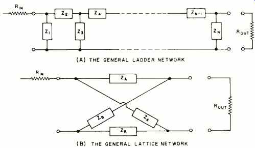
Fig. 2. (A) Unbalanced and (B) balanced arrangements.
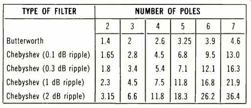
Table 1. Unloaded minimum "Q' " for two filter types.
Physical capacitors and inductors are not perfect. i.e., the best capacitors have sonic leakage and the best coils have some resistance. flow, there, may a filter be made which was designed assuming ideal elements? As a rule of thumb, it has been found that the more the filter requirements tighten, the less dissipation is allowable, and the closer the elements must be to the ideal. This is related to the elements by a term called the minimum "Q ". The ratio of reactance to resistance of a coil is called "Q ". When this ratio is small, the coil acts as an RL circuit and not like an inductor. This will put a large insertion loss in the filter passband and distort the passband shape, usually at the edges first. Because of this problem we must have a certain type of filter and a certain number of poles. Since the bandwidth may be vastly different for different designs, we normalize this information and allow it to be added later.
Table 1 is a list of the normalized unloaded "Q" required as a function of the number of poles and type of filter.
If the design is a low-pass type, these "Q's" are the minimum required for each element of the filter. If a band pass design is used, the normalized "Q" must be multiplied by the total filter "Q ". This, then, is the minimum "Q" required.
To illustrate how all of these aspects dovetail, let us design a filter for the band from 2 to 30 MHz with a v.s.w.r. of no greater than 1.5:1, an attenuation at least 35 dB at twice the-3 dB bandwidth at 50 ohms impedance. A v.s.w.r. of 1.5 represents a ripple of 0.177 dB (see Fig. 3) so a ripple of 0.1 dB is acceptable. The shape factor will be the limiting factor for the minimum number of elements we may use.
A good choice is a 5element Chebyshev, 0.1 dB ripple filter. See Fig. 4 below.
The normalized elements are found to be: L1 =1.15 µH, C2 =1.39 µF, L3= 1.97 pH, C4 =1.39 µF, and L5 =1.15 H.
De-normalizing by the following formulas gives us values for L' and C':
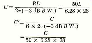
We get L' =0.327 pH, C2' =156 pF, L3' =0.560 µH, C4' =156 pF, and L5'= 0.327 uH. This gives us the low-pass prototype filter from which we can get the final bandpass design. This is achieved by resonating the low-pass elements at the geometrical mean frequency of the band we wish to filter, or
fo =__/ [f1 X f2 =__/ [2X30MHz] = 7.74 MHz
The additional elements required are thus found to be: C1' =1400 pF, L2'= 2.7 AFL C3' =725 pF, L4' =2.7 pH, and C5' =1400 pF.
The filter is of the ladder type and is shown along with its response in Fig. 4.
In practice, this filter would have to be built and aligned. To do this, certain changes are made. One is in the capacitors, two capacitors would be used, one fixed and the other a variable unit which could trim the fixed unit to the precise value required. The inductors would either be variable units or precision toroids: both could be pre adjusted on a "Q"-meter to the exact value and then installed.
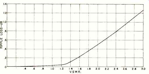
Fig. 3. The amount of loss due to ripple for various v.s.w.r.'s.
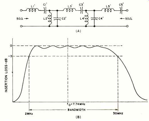
Fig. 4. The filter employed along with its frequency response.