By LAWRENCE S. NICKEL, Engineer, General Electric Co.
The harmonic content of various types of non-sinusoidal waves and the use of oscilloscopes to observe such waves.
WAVEFORM analysis is a complex field which can be very difficult to understand. Let's talk first about square waves, for instance. You may know that square waves have a lot of harmonics. What you may not know is that square waves have no even harmonics. Perhaps you know that the strength of the harmonics decreases as you go up in frequency.
For the square wave (with its 50% duty cycle, or "on" half of the time) this is certainly true, but for the pulse (other than 50% duty cycle), this is not necessarily so. Depending on the duty cycle, the fundamental or first harmonic may be strong, the next few harmonics decrease in strength, and then the following several harmonics may be stronger again.
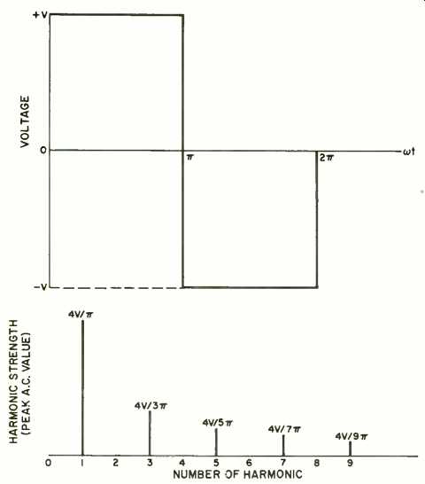
Fig. 1. The square wave at the top has a line spectrum (up through the
first nine harmonics) as shown at the bottom. Wave has no d.c. component,
hence no "O harmonic."
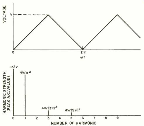
Fig. 2. Harmonic composition of triangular waveform. Note presence of
d.c. component and rapidly falling harmonics.
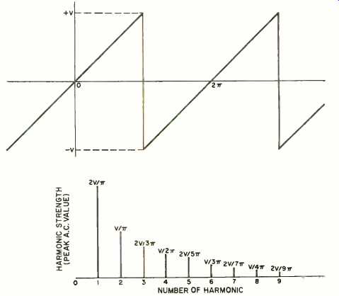
Fig. 3. This sawtooth waveform has the harmonics shown. Note that odd and
even harmonics are included in waveform.
We are concerned here with only periodic waveforms. A periodic waveform is one which repeats itself exactly each time interval, and this time interval is called the period.
Each periodic waveform which is non-sinusoidal will contain certain harmonics, the first of which is the fundamental. If the period is t (time), then the frequency f (in hertz) of the fundamental is 1 ft. No frequencies lower than the fundamental may be found in any complex waveshape.
A logical method for displaying the harmonic content of a waveform is by use of line-spectra charts. Refer to Figs. 1 through 3. These charts indicate the relative positions and strengths of each harmonic (only the first few harmonics are shown). Often a line is included at zero frequency to indicate the d.c. (average) value of the wave.
The set of harmonics are named Fourier series. According to theory the strength of the members (harmonics) of this series gets weaker and eventually goes to zero at infinite frequency. Since the waveform is actually the algebraic sum of all harmonics (which would include all those out to infinity), as we add higher and higher harmonics we get a closer and closer approximation of the actual waveform.
One way to predict the strengths of the harmonics of a particular waveform by using integral calculus; however, by using data with the harmonic strengths already worked out as shown in the figures, we can draw some conclusions. For instance, the ninth harmonic of a square wave is fairly weak compared with the lower harmonics.
This means that if your oscilloscope has a bandwidth approximately ten times the fundamental of the square wave, you can get a fairly accurate reproduction of the square wave on the scope screen. If your oscilloscope had a bandpass of up to 1 MHz with a very sharp cutoff there (which is unlikely) and you fed in a perfect 500-kHz square wave, you would see a 500-kHz sinusoid on the screen.
The shape of the waveform is directly related to its risetime. This is the time for the .value of the wave to go from 10% to 90% of its maximum value. In general, the faster the risetime, the stronger the higher harmonics. If the wave has sharp bumps or spikes, it will have strong harmonics up to many times the fundamental. There is also a correlation between sound and wave-shape. The waves with the sharp points (sawtooths, square waves, and triangular waves) are the ones that are rough or sharp sounding. The sine wave is the "smooth-sounding" one.
There is a relationship between bandwidth and risetime that is true for most oscilloscopes. The formula for expressing this is TrB =0.35, where Tr is the risetime of scope (µs) and B is bandwidth of scope (MHz). By knowing the risetime of your scope you can figure the approximate signal risetime it will display with little or no distortion.
Suppose you feed a pulse into your scope. If the risetime of the waveform is slow (long) with relation to the rise-time of the scope amplifier, then the scope will be able to reproduce the waveform accurately. But if the pulse has a risetime almost as short as or shorter than the oscilloscope's risetime, the scope amplifier will not be able to move the stored charge in the capacitors of the scope amplifier rapidly enough, and distortion occurs.
A simple formula relating the various rise-times is: t3= __/(t1^2+ t2^2), where t1 equals the scope risetime, t2 equals the actual signal risetime, and t3 equals the risetime which will be observed on the scope screen. Suppose the scope risetime is 3-µs. If a pulse is fed in with a 40-µs risetime, the observed risetime on the screen is almost exactly 40-µs.
So the scope has not distorted the pulse much. Suppose the wave put in has a risetime of only 4-µs; we will then see a pulse on the screen with a 5-µs rise-time. This risetime has been distorted or "stretched out" by 25%. Hence, we need to know risetime and frequency if we really want to know if the scope is giving a true picture.
=============
(adapted from: Electronics World magazine; Jul. 1975)
================