Test-equipment performance verification is an essential shop responsibility, because instruments must be accurate and in good working condition if they are to be a help instead of a hindrance at the bench.
The VOM and VTVM ( or TVM) are unquestionably the most basic test instruments. However, since these are well-known to practically all technicians, we will begin our coverage with the audio oscillator, which is the basic audio test instrument. The oscilloscope is also among the more basic test instruments; like the VOM, it is comparatively well known to the majority of technicians. Therefore, we will continue our coverage with the harmonic distortion meter and the intermodulation analyzer, which are among the more advanced specialized audio instruments. The Section concludes with a practical discussion of tone burst generator characteristics and performance verification procedures.
GENERAL DISCUSSION
Service-type audio oscillators are often rated for less than 1 percent harmonic distortion. A few instruments are rated for less than 0.5 percent distortion; however, the lower-priced instruments are rated in the order of 5 percent distortion. In some cases, a distortion rating applies over less than the complete frequency range. For example, an audio oscillator that has a frequency range from 20 Hz to 1 MHz might have a distortion rating of less than 0.25 percent from 20 Hz to 20 kHz, with no rating from 20 kHz to 1 MHz. To measure the percentage of distortion in an audio-oscillator output signal, feed the signal directly into a harmonic-distortion meter, as shown in Fig. 8-1. A scope is optional, but is useful to determine whether the distortion is chiefly second-harmonic or third-harmonic. A scope also helps in analyzing possible hum in the signal.
The flatness of output over the complete range of the audio oscillator can also be checked with a scope.
Harmonic-distortion measurements should be made at several intervals; for example, measurements may be noted at 20, 200, 2000, and 20,000 hertz.
The values indicated by the HD meter might not be accurate if there is a defect in the instrument. There fore, it is good practice to cross-check with another HD meter, if possible. In case both HD meters are in agreement, it is generally safe to conclude that both meters are accurate. If the scope is deflected at a horizontal rate that displays one cycle when the HD meter is operating on its Set Level function (display of the fundamental output from the audio oscillator), harmonics are identified as follows when the HD meter is set to read percentage of distortion. If the distortion pattern displays two cycles on the scope screen, we know that second-harmonic distortion is present. Or, if the distortion pattern displays three cycles on the scope screen, we know that third harmonic distortion is present.
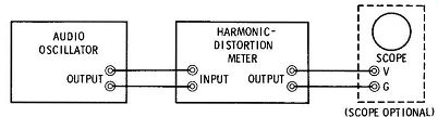
Fig. 8-1. Harmonic-distortion check of audio oscillator.
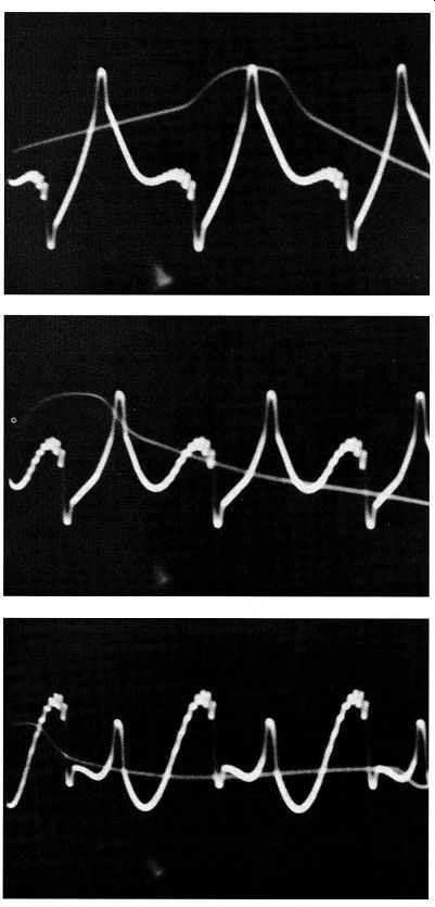
Fig. 8-2. Typical change in shape of a harmonic-distortion waveform as
the harmonic-distortion meter is tuned through the null point.
In many cases, the distortion products from an audio oscillator will be a combination of second- and third-harmonic components. In such a case, the peaks in the waveform will have unequal heights; the number of cycles in the pattern will depend on whether the second harmonic or the third harmonic is predominant. Higher-order harmonics may be perceptible also but they are usually quite small in relative amplitude. The scope pattern will change as the HD meter is tuned through the null point, as illustrated in Fig. 8-2. In this example, the second photo shows the true distortion-product pattern, with the HD meter reading at the null point. Hum will show up as a blurring of the distortion pattern, except when the HD meter is operated at 60 Hz or 120 Hz. If tuned slightly to one side of 60 or 120 Hz, hum voltage causes a "writhing" of the distortion pattern; the needle will also be seen to "wiggle" on the HD meter.
If the measured percentage of distortion is out of rating for the audio oscillator, the trouble may be due to excessive power-supply ripple, as noted above.
The filter capacitors are usually the offenders in this case. On the other hand, if the B+ ripple is negligible, the tubes should be checked or replaced. In the majority of cases, these simple procedures will bring the percentage of distortion within its rated value. However, if the difficulty persists, the next step is to check the circuit capacitors for leakage or opens.
Note that in very-high-resistance bridge circuits, such as employed in some audio oscillators, even a slight amount of capacitor leakage will seriously up set the bridge operation. For example, resistors with values up to 18 megohms may be used on the first range. Fig. 8-3 shows a simplified circuit diagram for a Wien-bridge oscillator.
Resistors are less likely to cause trouble in an audio oscillator than are capacitors. However, resistors will occasionally become defective. In tube-type instruments, resistors may become damaged by excessive current due to tubes that develop inter electrode shorts. This source of trouble is much less common in transistorized audio oscillators, even if a transistor develops a "dead" collector-to-base short.
That is, the supply voltages are much lower in a solid-state instrument, which generally eliminates the possibility of burned resistors. Composition resistors tend to drift in value with age, and the general tendency is for the resistance value to creep upward. However, there are exceptions, and most technicians can recall situations in which a resistor was found to have decreased in value.
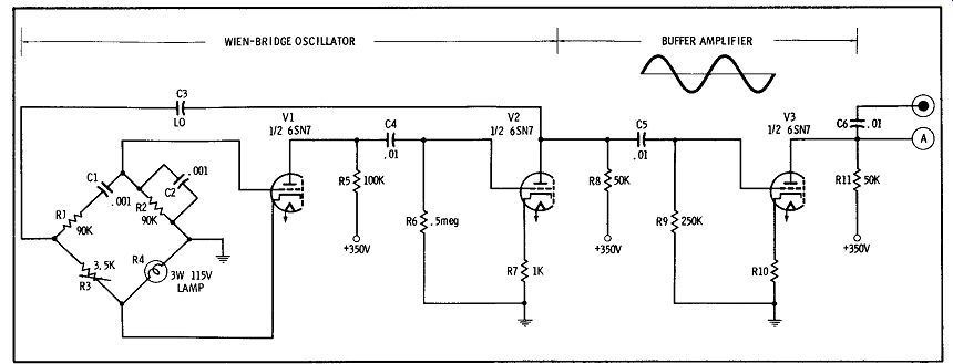
Fig. 8-3. Basic Wien-bridge oscillator configuration.
Next, let us consider frequency-calibration requirements. The tuning dial of an audio oscillator is usually rated for calibration accuracy, and all instruments have trimmer capacitors or some equivalent provision for frequency adjustment. Fig. 8-4 shows a practical shop-test setup for low-frequency calibration of an audio oscillator. The 60-Hz power line is used as a frequency reference. Although a single frequency check might not have extremely high accuracy, the long-time accuracy of the 60-Hz power frequency is very good. Therefore, we can make several frequency checks at separated intervals, and take the average to maximize the accuracy of measurement. Zero beat is displayed as a Lissajous pattern; the 60-Hz Lissajous figure is illustrated in Fig. 8-5. Its aspect depends upon the phase relation of the two input voltages; if the audio oscillator is tuned slightly off zero beat, the pattern slowly progresses through its various aspects.
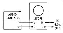
Fig. 8-4. Low-frequency calibration test setup.
When the dial of the audio oscillator is tuned to 120 Hz, the Lissajous pattern has the form pictured in Fig. 8-6; its aspect depends on the phase relation of the two input voltages. A summary of basic patterns for various frequency ratios is seen in Fig. 8-7. We will observe that the ratio of the two input frequencies is given by the points of tangency in a Lissajous figure. Thus, we write:
where, f11 is the frequency applied to the horizontal input, fv is the frequency applied to the vertical input, nv is the number of points at which the pattern is tangent to a vertical line, nh is the number of points at which the pattern is tangent to a horizontal line.
With reference to Fig. 8-8, observe that the Lissajous figure touches vertical line B-B at two points ( 4 and 16) , and touches horizontal line A-A at three points (5, 13, and 21). The frequency ratio in this example is 2: 3. For example, if the frequency applied to the vertical input is 60 Hz, the frequency applied to the horizontal input is given by: t = ¾ X 60 = 40 Hz The National Bureau of Standards maintains WWV transmissions on carrier frequencies from 2.5 to 25 MHz, with audio modulation frequencies as tabulated in Fig. 8-9. To check the calibration of an audio oscillator against the 440- or 600-Hz WWV modulation frequencies, simply tune in the signal on a radio receiver and feed the speaker voltage to the input terminals of a scope. Then, spot-checks of numerous frequencies can be made by means of Lissajous figures as has been explained. This procedure becomes more critical as we proceed to check higher audio frequencies, since a very slight movement of the tuning dial then changes the audio oscillator frequency appreciably. A vernier tuning control is helpful in this regard.
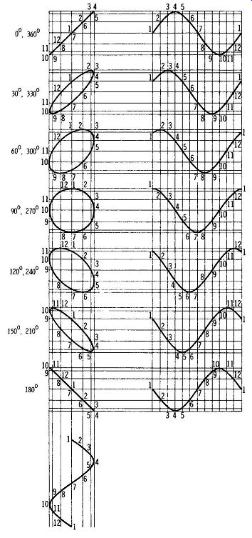
Fig. 8-5. Effect of phase difference on pattern aspect.
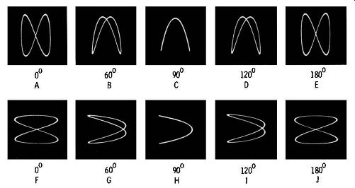
Fig. 8-6. Lissajous pattern for a 2:1 frequency ratio.
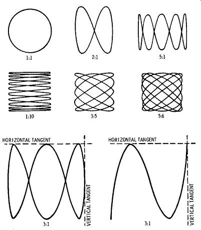
Fig. 8-7. Lissajous patterns 'for various frequency ratios.
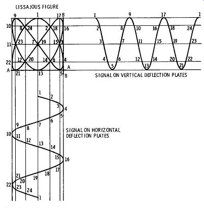
Fig. 8-8. In-phase Lissajous pattern for a 2:3 frequency ratio.
FLATNESS OF OUTPUT
Most audio oscillators are rated for uniformity of output amplitude (flatness). For example, a typical instrument has a rating of ±1.5 dB over its entire frequency range. It was previously explained how the uniformity of output can be checked with a scope; this procedure assumes that the scope has a frequency response that is quite flat. Alternatively, an ac VTVM can be used. Remember to check each band on the audio oscillator. If the VTVM has a dB scale, checking of flatness ratings is thereby facilitated. We are not concerned with the specific dB level, but with the number of dB of variation over the frequency range of the audio oscillator. Thus, it is convenient to adjust the output level so that the dB meter indicates 0 dB at 1 kHz. Then, if the maximum observed variation is between the limits of + 1 and -1.6 dB on the scale, the total variation is 2.6 dB, which can be expressed as ±1.3 dB, or as + 1 and -1.6 dB with respect to 1 kHz. It is good practice to check an audio oscillator under rated load, because the flatness may vary somewhat when the load is other than the rated value.
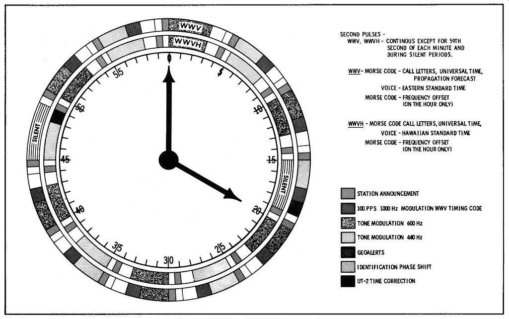
Fig. 8-9. WWV and WWVH transmissions. SECOND PULSES -
WWV, WWVH - CONTI NOUS EXCEPT FOR 59TH SECOND OF EACH MINUTE AND DURING SILENT PERIODS. WWV- MORSE CODE - CALL LETTERS, UNIVERSAL TIME, PROPAGATION FORECAST VOICE - EASTERN STANDARD TIME MORSE CODE - FREQUENCY OFFSET ION THE HOUR ONLY) WWVH - MORSE CODE CALL LETTERS, UNIVERSAL TIM£, VOICE-HAWAIIAN STANDARD TIME MORSE CODE - FREQUENCY OFFSET (ON THE HOUR ONLY)
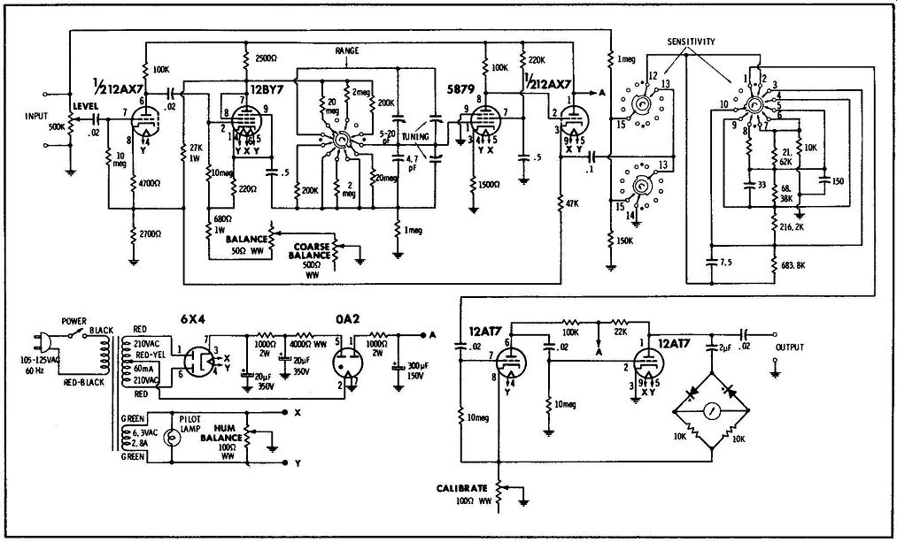
Fig. 8-10. Circuit diagram of a typical harmonic-distortion analyzer.
HARMONIC-DISTORTION METER
The configuration for a typical harmonic-distortion meter is shown in Fig. 8-10. This instrument comprises a high-gain VTVM with a tuned RC-type rejection filter. Switching facilities are provided so that the meter can be operated either with or without the rejection filter. In this example, the VTVM has full-scale ranges of 1, 3, 10, and 30 volts rms. The meter responds to the average value of a waveform because instrument rectifiers are employed-the meter scales are calibrated in rms values. A 500-k potentiometer serves as the input set-level control; this is an operating control. The coarse-balance control is a maintenance adjustment-it is set to a point that gives an average setting of mid-range for the balance control, which is an operating control.
Note that the sensitivity (range) switch in Fig. 8-10 is basically a VTVM multiplier, and is an operating control. Frequency-compensating capacitors are included in the multiplier network to provide flat response from 20 Hz to 20 kHz. The accuracy of full-scale VTVM indication is adjustable by means of the 100-ohm calibrate control. In practice, calibration is usually made by feeding the output from an audio oscillator to the harmonic-distortion meter and to a VTVM that is known to be reasonably ac curate. Then, the calibrate control in the HD meter is adjusted to provide the same scale indication as the VTVM. Note in Fig. 8-10 that a hum-balance control is also provided; this is a maintenance control. It is adjusted by switching in the rejection filter while the HD meter is being driven by an audio oscillator. The filter is tuned for minimum indication on the meter, and the hum-balance control is then adjusted to reduce the reading still farther, if possible.
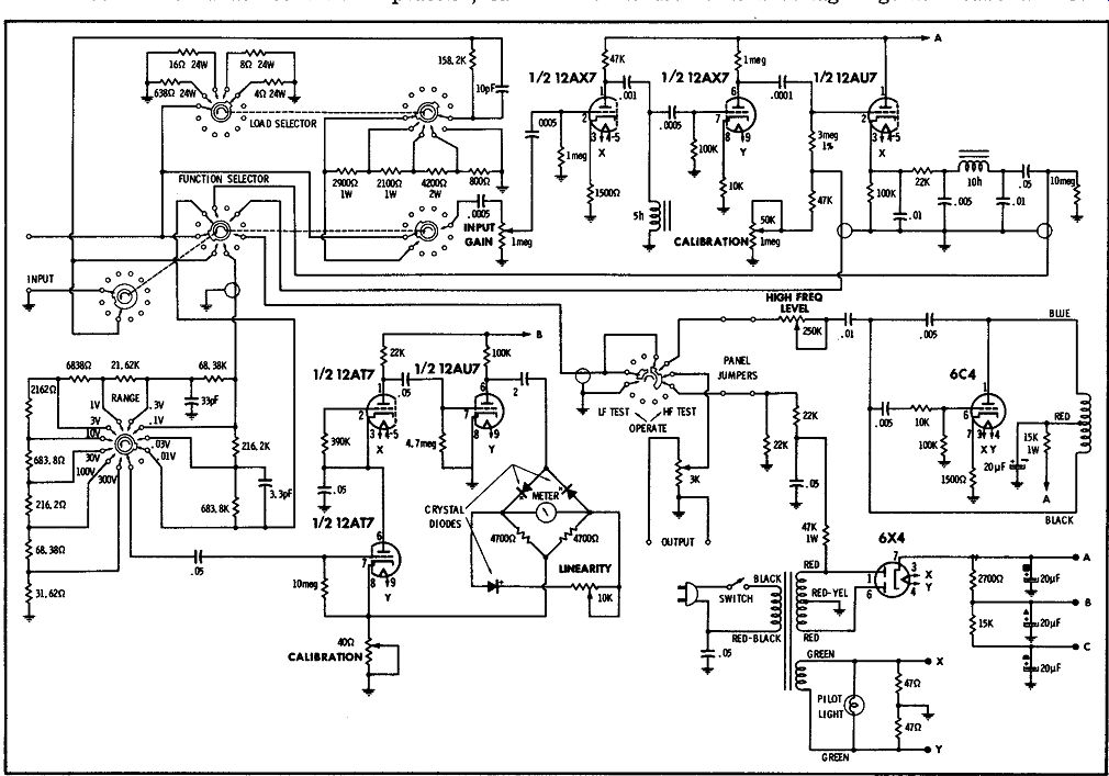
Fig. 8-11. Circuit diagram of a typical intermodulation-distortion analyzer.
Most trouble symptoms in harmonic-distortion meters are caused by defective tubes. As in the case of many other electronic instruments, capacitors are the next most likely suspects. Although semiconductor instrument rectifiers are normally long-lived, they will fall under scrutiny if the calibrate control is out of range. As in all quantitative-indicating instruments, the power supply must be well regulated; if the meter calibration tends to drift, monitor the B+ voltage to see if it varies from time to time.
Remember that a voltage-regulator tube will continue to glow, although it might be nearing the end of its useful life as its regulating action becomes progressively poorer.
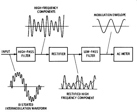
Fig. 8-12. Basic configuration and waveforms in an intermodulation-distortion
analyzer.
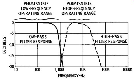
Fig. 8-13. Characteristics of the filters in a typical inter modulation-distortion
analyzer.
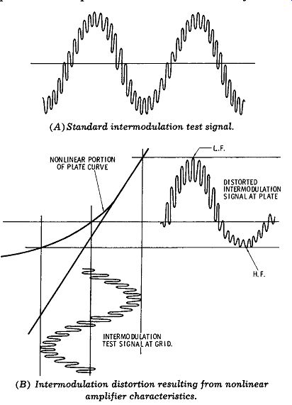
Fig. 8-14. Test signal and results of intermodulation-distortion test of
a nonlinear amplifier. (A) Standard intermodulation test signal. (B) Intermodulation
distortion resulting from nonlinear amplifier characteristics.
INTERMODULATION ANALYZER
Intermodulation analyzers are somewhat more complicated instruments than harmonic-distortion meters, and are less widely used in hi-fi service shops for this reason. However, IM analyzers are used in all professional and engineering laboratories.
A circuit diagram for a service-type IM analyzer is shown in Fig. 8-11. The indicating meter operates in a basic VTVM configuration. The plan of the instrument is shown in Fig. 8-12. The signal channels employ two filters with high- and low-pass characteristics as shown in Fig. 8-13; these filters separate the IM distortion products from the input waveform.
These distortion products are generated as the result of nonlinearity, as shown in Fig. 8-14.
It is helpful to review briefly the operation of an IM analyzer. A built-in 6-kHz oscillator generates the high-frequency component of the test signal, and a 60-Hz voltage from the power line serves as the low-frequency component. This is called a two-tone test signal, and has the normal waveform shown in Fig. 8-14A. The two-tone signal is available at the output terminals in Fig. 8-11, and it can be checked with a scope. Note that the low-frequency level is fixed, but the relative amplitude of the high-frequency component is adjustable by means of a maintenance control (High Freq. Level) . An amplifier or device under test for intermodulation distortion is driven by this two-tone signal. If the transfer characteristic of the amplifier or device is perfectly linear, the two-tone signal is undistorted; in other words, no distortion products are formed.
Next, let us consider the situation in which the amplifier or device under test has a nonlinear characteristic. In this case, the two-tone signal will have one peak region compressed, as shown in Fig. 8-14B. This is an intermodulation process that results from a nonlinear transfer characteristic, and its effect is to modulate the low-frequency signal on the high frequency signal, as shown in Fig. 8-12. This modulated waveform from the amplifier under test is applied to the input terminals of the IM analyzer in Fig. 8-11. With reference to Fig. 8-12, the signal flows first through the high-pass filter, which removes the 60-Hz component and leaves the modulated signal. This modulated signal is next rectified in a detector circuit that develops the rectified high frequency component. The demodulated signal then flows through a low-pass filter which develops the low-frequency modulation envelope. The amplitude of this envelope waveform is proportional to the percentage of intermodulation distortion, which is indicated by the VTVM section of the IM analyzer.
The indicating meter in a service-type IM analyzer is an average-indicating type employing semiconductor-diode instrument rectifiers. In the example of Fig. 8-11, a linearity diode is also provided. The VTVM calibration control is a maintenance adjustment, and is set in the same manner as previously explained for a harmonic-distortion meter. It interacts to some extent with the Linearity control, which is a maintenance adjustment. The Linearity control is set to a point that provides best scale-indication consistency when the VTVM multiplier is dropped down one step. We work back and forth between the two controls to obtain accurate full-scale indication and accurate %-scale indication.
Since the Input Gain potentiometer is an operating control, it requires no attention unless it becomes defective. The IM Calibration control is a maintenance control, and it requires due attention if the accuracy of the IM measurements is to be retained as tubes age and components drift. This IM analyzer calibration can be carried out in various ways. In any case, a signal that involves 10 percent IM distortion is applied to the analyzer section, and after the input control is adjusted to produce full-scale reading on the 1 percent IM range, the IM control is then set for full-scale reading on the Set Level positions of the Function and Range switches.
A satisfactory method of IM-analyzer calibration, using a minimum of equipment, requires an audio oscillator and a pair of resistors of approximately 10-k each. A signal that will produce 10 percent IM distortion can be formed by mixing the signal from the IM generator section in this example with the signal from the audio oscillator in a voltage ratio of 10: 1, and with a frequency difference of 60 to 100 Hz. We make up the calibrating resistor network by connecting the 10-k resistors to a 4.7-k resistor, as shown in Fig. 8-15. The test switch on the IM analyzer is set to the HF Test position, so that the 60-Hz signal is removed from the two-tone output, leaving only the 6-kHz component. With reference to Fig. 8-15, some connections are shown in dotted lines, and other connections are shown in solid lines.
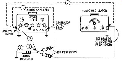
Fig. 8-15. Calibration resistor arrangement.
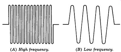
Fig. 8-16. Tone-burst waveforms. (A) High frequency. (B) Low frequency.
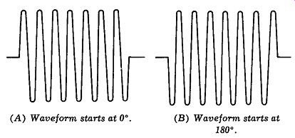
Fig. 8-17. Noncoherent bursts. (A) Waveform starts at 0°. (B) Waveform
starts at 180°.
The solid-line connections are used throughout the calibration procedure, whereas the dotted-line connections are used only in certain portions of the procedure.
Next, we check the IM calibration as follows: Connect one of the matched resistors from the "hot" output terminal of the IM analyzer to the 4.7-k resistor, and connect the other end of the 4.7-k resistor to ground. The other matched resistor is connected from the audio-oscillator output terminal to the same 4.7-k resistor, and thence to ground. The IM analyzer is operated in the VTVM mode, with the load switch turned to the Hi-Z position. We set the Input Gain and the Generator Output controls to minimum; the range switch is set to 10 volts, and the input terminal of the IM analyzer is connected to the junction of the three resistors, as denoted by the dotted line No. 3 in Fig. 8-15.
Next, the audio oscillator is tuned for zero-beat with the output from the analyzer. This part of the procedure requires that the High-Frequency Level and Generator Output controls be set to maximum.
Using maximum output from the audio oscillator, watch the pointer as the audio oscillator is tuned through 6 kHz. The dial is carefully adjusted for zero beat (motionless pointer). Then, remove connection No. 3 in Fig. 8-15, and set the audio oscillator to a frequency that is 60 to 100 Hz higher or lower than the zero-beat setting. Make the two No. 1 connections as follows: Short the 4.7-k resistor and connect the input terminal to the IM analyzer signal-output terminal. Adjust the High-Frequency Level and Generator Output controls to indicate a maximum value on the 30-volt range of the meter.
Remove the No. 1 connections in Fig. 8-15 and make the No. 2 connections, shifting the input terminal lead from the output of the IM analyzer to the output of the audio oscillator. Then, adjust the output control on the audio oscillator to obtain the same meter deflection as noted above, except that now the meter is operated on its 3-volt range.
In this manner, establish a voltage ratio of 10: 1.
Now remove the No. 2 connections and make the No. 3 connection. This takes the short-circuit away from the 4.7-k resistor and connects the input of the IM analyzer to the junction of the three resistors.
Making these connections results in applying the desired mixed signal to the analyzer and will result in a carrier with 10 percent modulation at the detector in the analyzer. Set the range switch to its 10 percent IM position, and set the function switch for measurement of percentage of IM. Then, adjust the IM Input Gain control for full-scale meter deflection. The function switch is turned to its Set Level position, and the Range switch is set to the indicated Set Level position (3 percent IM). Finally, adjust the IM Calibrate control for full-scale meter deflection, and the procedure is completed.
TONE-BURST GENERATOR
A tone-burst generator provides a sine-wave output that is keyed on and off at regular intervals.
The frequency of the sine wave is ordinarily adjust able to any value in the audio range. Fig. 8-16 shows a pair of ideal tone-burst waveforms. Since tone burst generators are comparatively expensive instruments, they are used chiefly in engineering labs.
Although it is easy to connect an audio oscillator to an electronic switch in order to generate a tone-burst waveform, there is a basic disadvantage to this simple method. That is, the sine wave does not start at the same point in successive bursts, as shown in Fig. 8-17. When the sine wave starts at random phases in successive bursts, the waveform is said to be noncoherent. To generate a coherent tone-burst waveform, the gating circuit (electronic switch) must be tightly locked to the sine-wave frequency.
It is desirable to employ a coherent tone-burst waveform, because the transient response of an amplifier or speaker depends on the polarity of the first excursion in the sine wave, and also on the exact phase of the starting point. If a coherent tone burst generator is checked by feeding its output into a scope, the following waveform characteristics are observed in normal operation:
1. There is no blurring in the burst display, and there is negligible jitter.
2. The burst has a good sine waveform, with level top and bottom peaks.
3. No DC component is evident; that is, the burst is centered on the horizontal axis.
4. Stability is maintained over the entire audio frequency range; the tone burst does not blur at certain critical frequencies.
5. Rise time is sufficiently fast that there is negligible distortion of the first half-cycle in the burst, even at high audio frequencies.
6. The tone burst ceases abruptly, without noticeable ringing.