Guide to LC Circuits--FUNDAMENTAL THEORY

This Section digests those parts of basic electronics that are essential to an understanding of inductance-capacitance (LC) circuits. These are specific items requiring for their understanding a general familiarity with electrical theory and the mathematics of electronics, and it is assumed that the reader has that background.

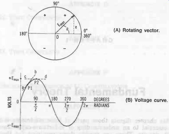
Fig. 1. Development of sine wave.

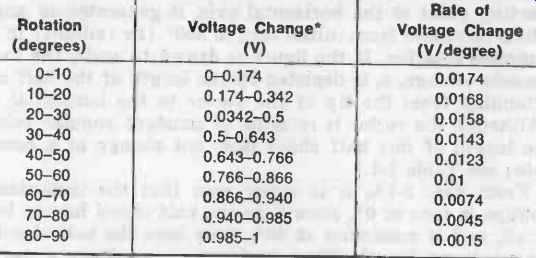
Table 1. Voltage Change and Rate Change

1. THE AC CYCLE-RATE OF CHANGE

Fig. 1A depicts a sinusoidal ac voltage in terms of a vector rotating at constant velocity. The magnitude of this vector is Emax, the maximum value attained by the ac voltage.

As the vector moves in a counterclockwise direction from its starting point at the horizontal axis, it generates an angle 0 which increases from initial zero to 360° (2 pi radians) in each complete rotation. If the figure is drawn to scale, the instantaneous voltage, e, is depicted by the length of the half chord extending from the tip of the vector to the horizontal axis.

(Although the vector is rotating at constant angular velocity, the length of this half chord does not change at a constant rate; see Table 1.) From Fig. 1A, it is easily seen that the instantaneous voltage is zero at 0°, since here the half chord has no length at all, and is maximum at 90°, since here the half chord has its maximum length. Thus, instantaneous voltage e starts at zero, increases to the maximum positive value (+Emax) at 90° (pi /2 radians), returns to zero at 180° ( pi radians), increases to the maximum negative value (-Erna.) at 270° (3 pi /2 radians), and returns to zero at 360° (2 pi radians). At this latter point, the vector has traced out a complete cycle, and a new cycle begins with the continued rotation of the vector. The length of line e, and accordingly the value of the instantaneous volt age, is proportional to the sine of angle 0, and for a circle of unit radius (i.e., E. = 1), it is equal to sin 0. The value of instantaneous voltage at any point, therefore is :

e = Emax sin theta (1-1)

Fig. 1B shows the familiar plot of instantaneous voltage versus angle. This curve is identical with that of the sine function from trigonometry, hence the term sine wave (or sinusoidal).

Illustrative Example: The 115-V power-line voltage has a maximum (90°) value of 162.6 volts. Calculate the instantaneous value at 60°. Sin 60° = 0.866.

From Equation 1-1, e = 162.6 (0.866) = 140.8 V.

A close examination of Fig. 1 shows that not only is the instantaneous voltage continuously changing during the cycle, but the rate of change also is changing. (See Column 3 in Table 1.) This can be shown graphically by drawing tangents to the curve at points of interest and observing the slope of the tangent. Thus, in Fig. 1B, the tilt of tangent ab at Point P1 (45°) reveals a moderate rate of change, whereas tangent cd at Point P2 (90°) has no tilt whatever and shows that there is no change at all at this point. In the sine-wave cycle, the rate of change thus is zero at 90° and 270° when the cycle is passing through its maximum points, and is maximum when the cycle is passing through its zero points (0°, 180°, and 360°).

This can be shown mathematically : (1) The increment of voltage around the point of interest divided by the increment of the angular rotation at that point equals the slope ; thus, slope = AE/00. From Fig. 1B, it is easily seen that at 90° (Point P2), AE = 0, and the slope and rate of change accord ingly are zero, whereas at 180° AE is very large for a small value of AO, so the slope is steep at this point and the change is great. (2) From calculus, the rate of change of a sine wave at a point of interest is proportional to the cosine of the angle at that point. The cosine of 90° or of 270° is zero, so the rate of change is zero at those points. The cosine of 0° and of 360° is 1, so the rate of change is maximum at those points where the cycle crosses the zero line (the maximum value of the co sine function is 1).

At a given frequency f, the voltage vector describes 2 pi f radians per second (where f is in hertz, and π = 3.1416). The expression 2 pi f is often represented by lowercase Greek omega : ω. (Appendix A gives values of omega at a number of frequencies between 1 Hz and 100 MHz.) The maximum rate of change in voltage is equal to 2 pi f Emax. (also written omega Emax.), and it follows from the previous discussion that this rate of change must occur at zero-voltage points in the cycle. At every point, the rate of change may be found by multiplying the maximum rate of change by the cosine of the angle at the point of interest:

Rate of Change = 2 pi f Emax cos θ = omega Emax cos θ (1-2)

For example, in a 500-Hz cycle having a maximum voltage of 15 V, the rate of change at 65° (where cos θ = 0.42262) is 2 (3.1416)500 (15) 0.42262 = 19,915 volts per degree. At 0° (where cos θ =1), the rate of change is 2(3.1416)500 (15)1 = 47,124 volts per degree. At 90° (where cos θ = 0), the rate of change is 2(3.1416)500 (15)0 = 47,124 x 0 = 0 volts per degree.

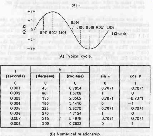
Fig. 2. Illustrative cycle. (A) Typical cycle. (B) Numerical relationship.

Fig. 2A illustrates a specific example. This is one cycle of 125-Hz ac voltage having a maximum value of 2 volts. The horizontal axis is divided into seconds of time, instead of degrees, but these time units are easily converted into an angle, if desired :

0 = 2 pi ft = wt (1-3)

where, is the angle in radians, f is the frequency in hertz, t is the time in seconds, is 3.1416, w is an-f.

To convert 0 to degrees, multiply by 57.296. To obtain degrees directly, change Equation 1-3 to :

theta = 360 ft (1-4)

Fig. 2B shows the relationship between selected angles and time instants, and gives sines and cosines of these angles.

Note the rate of change exhibited in this cycle. The maximum rate of change here (271-fErna0 is 1570.8 V/s. From Equation 1-2, the rate of change at 0.004 second (180°, 7T radians) is 2 (3.1416) 125 (2) (-1) = 1570.8 (-1) =-1570.8 V/s ; the rate of change at 0.001 s (45°, pi /4 radians) is 2 (3.1416)125 (2) 0.7071 = 1110.7 V/s ; and the rate of change at 0.002 s (90°, pi /2 radians) is 2(3.1416)125 (2)0 = 1570.8 x 0 = 0.

It should be clear by now that the rate of change in voltage at a selected point in the ac cycle is markedly different in magnitude from the instantaneous voltage at that point. In the preceding example, for instance, it is seen that the instantaneous voltage at the 0.001-second point (45°) is (from Equation 1-1) 2 x sin 45° = 2(0.7071) = 1.414 V; but the rate of change of voltage at that point (from the foregoing paragraph) is 1110.7 volts per second. The various aspects of rate of change in the ac cycle must be mastered and remembered, since a clear understanding of inductor and capacitor operation and of LC circuits demands this comprehension.

What has been said in this section about ac voltage and the voltage cycle applies equally well to ac current and the current cycle. It is necessary only to substitute the word current for voltage, and the symbols I and i for E and e in the discussion.

2. NATURE OF RESISTANCE

It is necessary to introduce a discussion of resistance at this point, since internal resistance is unavoidable in inductors and capacitors and can influence the performance of LC circuits.

Resistance (R or r) is the simple opposition offered to the flow of an electric current. It is somewhat analogous to the friction encountered by flowing water. Resistance is directly proportional to voltage and is inversely proportional to cur rent, as shown by Ohm's law :

R = I (1-5)

where, R is the resistance in ohms, E is the voltage in volts, I is the current in amperes.

An applied voltage E thus will force a current I = E/R through a resistance R; likewise, a current I through a resistance R will produce a voltage drop E = IR across the resistance.

While all conductors of electricity exhibit some resistance, however tiny, resistance is primarily the property of resistors. Resistance is measured in ohms and in multiples and submultiples of the ohm (See Table 1-2).

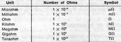
Table 2. Units of Resistance

Conventional (ohmic) resistors are made principally from suitable metals in the form of wire, strip, ribbon, or film; from carbon or graphite; and from certain controllable-resistivity compositions, mixtures, and oxides. Nonlinear (non-ohmic) resistors, whose resistance depends upon applied voltage, and thermistors, whose resistance depends upon temperature, are made from semiconductors or from suitable com pounds, such as complex oxides. In addition to discrete resistors, there are integrated resistors which are processed into integrated circuits (ICs) . Variable, as well as fixed, resistors are readily obtainable, and all resistors are available in a wide range of resistance and power ratings, shapes, and sizes. For special purposes, the internal resistance of some other device--such as a vacuum tube, transistor, semiconductor diode, or filament-type lamp-is sometimes employed instead of a resistor per se.

Pure resistance introduces no phase shift. Fig. 3 illustrates this zero-phase-shift feature; in both the wave plot (Fig. 3B) and the vector diagram (Fig. 3C) , current and volt age are in step at all points. Because pure resistance is impossible to attain in practice, all resistors possess some inherent inductance and capacitance, but these extraneous properties are usually, but not always, so minute that they can be ignored.

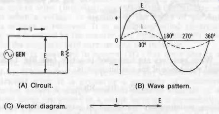
Fig. 3. Phase relationship: resistance.

Resistance is a dissipative property : that is, resistors consume power. Current (I) flowing through resistance (R) causes heat to be generated in the resistor, just as mechanical friction gives rise to heat in bodies rubbed together. In this way, electrical energy is converted into heat energy, and the latter represents energy that is lost for some intended electrical work. The electrical loss is power dissipation and may be expressed as :

P=I^2 R (1-6)

where, P is the power loss in watts, I is the current through the resistance in amperes, E is the voltage across the resistance in volts, R is the resistance in ohms.

The sine-wave pattern shown in Fig. 4 shows resistor power in relation to current and voltage.

When operated within their ratings, good-grade conventional resistors undergo very little change in resistance as a result of variations in voltage, temperature, or frequency.

Exceptions are voltage-dependent resistors (vdr's) , which are designed to be voltage sensitive, and thermistors, which are designed to be temperature sensitive.

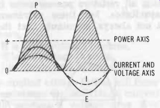
Fig. 4. Power in resistor.

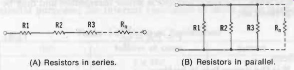
Fig. 5. Basic resistor circuits. (A) Resistors in series. (B) Resistors in parallel.

When resistors are connected in series (see Fig. 5A), the total resistance of the combination is :

Rt R1 + R2 + R3 + . . . + (1-7)

When resistors are connected in parallel (Fig. 5B) , the equivalent resistance of the combination is :

Req = 1 /[ [1/R + 1/R2 + 1/ R3 ... 1/Rn ](1-8)

If only two resistors are connected in parallel, the equation can be simplified to R = (R1R2) / (R1 + R2) . If n resistors, each having the same value R, are connected in series, the total resistance of the combination is R, = nR. If n resistors, each having the same value R are connected in parallel, the equivalent resistance of the combination is Re, = R/n.

Table 1-3. Units of Inductance

3. NATURE OF INDUCTANCE

Inductance (L) is the property exhibited by a conductor or by a coil of wire (inductor) which retards the buildup of current when a voltage is applied, or the decay of current when a voltage is removed. It is sometimes called electrical inertia, and is caused by the counter emf ("back voltage") produced by the magnetic field surrounding the inductor.

Inductance is measured in henrys (H) ; but since this is a large unit, submultiples of the henry are often used (see Table 1-3). While inductance is present in any conductor, even in a straight wire, it is primarily a property of inductors (also called coils). A simple practical inductor consists of a coil whose turns are wound in a single layer on a nonmetallic, cylindrical form and its inductance (L) depends upon the number of turns (N), the length of the coil (1), and the diameter of the coil (d) :

L = 0.2 d^2 N^2 / 3d + 91 (1-9)

where, L is the inductance in microhenrys, d is the diameter of the winding in inches, 1 is the length of the winding in inches, N is the number of turns.

The inductance formula becomes somewhat different when the inductor is wound in several layers or when it is wound on a core of magnetic material (iron, steel, ferrite, etc.) .

The core and the multilayer winding (increased number of turns) each increases the inductance (the higher the permeability--,a-of the core material, the fewer the turns needed for a given inductance). Inductors are manufactured in a wide range of inductance, current, voltage, and internal-resistance ratings and in numerous shapes and sizes. Inductors are available in fixed and variable types.

Inductance is also found in places other than in inductors.

It is inherent in other components and devices than inductors.

For example, by their nature transformer windings have inductance, and so do the leads of capacitors, resistors, and other components. Even short, straight wires exhibit inductance, which-though tiny-can be deleterious at very high frequencies.

All inductors have internal resistance (R) which at de and low frequencies is due to the resistance of the wire. At higher frequencies, other factors-such as core losses and skin effect-combine with the wire resistance to determine the total resistance of an inductor. In a high-quality inductor, resistance, which acts in series with the inductance, is held to a minimum.

When a de voltage is applied to an inductor, the resulting final current is determined by the resistance of the winding.

But the current does not reach this value at once, nor can it be rapidly increased or decreased. Any such change is opposed by the counter emf, which is opposite in polarity and is produced by the surrounding magnetic field. This means that the current does not even begin to flow until a short time after application of the voltage. Thus, current lags voltage (voltage leads current) in an inductive circuit.

Because of the action just described, pure inductance would introduce a 90° phase shift in an ac circuit. Fig. 6 illustrates this 90°-lagging phase feature. In both the wave plot (Fig. 6B) and the vector diagram (Fig. 6C), current and voltage are out of step by 90° at all points. Examination of Fig. 6B shows that maximum inductor current flows when the rate of change in voltage is maximum (that is, when the ac cycle is passing through zero) ; and, conversely, inductor current is zero when the rate of change in voltage is zero (that is. when the ac cycle is at maximum). For a clarification, see Section 1.1 for a discussion of rate of change. Because pure inductance is impossible to attain in practice, all inductors possess some inherent resistance and capacitance and these extraneous properties are usually small. Nevertheless, inherent resistance (internal losses) prevents a practical inductor from introducing full 90° phase shift.

Pure inductance, unlike resistance, consumes no power. This results from energy being stored in the magnetic field during one half-cycle (when the field is expanding) and being re turned to the ac generator during the next half-cycle (when the field is collapsing) . The wave pattern in Fig. 7 depicts inductor power (for an ideal inductor) in relation to current and voltage (compare with Fig. 4, the wave pattern for resistor power, and Fig. 11, the wave pattern for capacitor power). Note that the frequency of the power wave is double that of the current wave or the voltage wave. In a practical inductor, the only power loss is that associated with the internal resistance of the inductor.

(A) Circuit. (B) Wave pattern. (C) Vector diagram.

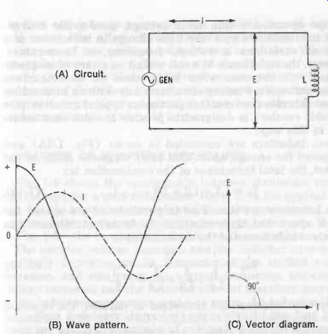
Fig. 6. Phase relationship: inductance.

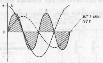
Fig. 7. Power in ideal inductor.

When operated within their ratings, good-grade conventional inductors undergo very little change in inductance as a result of variations in voltage, frequency, or temperature. However, the inductance of a coil wound on a core of magnetic material will decrease when high values of direct current flowing through a winding simultaneously with an alternating current saturate the core. One particular type of inductor (the saturable reactor) is designed to provide dc-controlled inductance in this way.

When inductors are connected in series (Fig. 8A) and are spaced far enough apart that their magnetic fields do not interact, the total inductance of the combination is :

Lt = L1 + L2 + L3 + . (1-10)

When inductors are connected in parallel and are spaced far enough apart that their magnetic fields do not interact, the equivalent inductance of the combination is :

Leq = 1 1 1 1 1 L1 L2 L3 L

If only two inductors are connected in parallel, the equation can be simplified to L = (L1L2) / (L1 + L2). If n inductors, each having the same value L, are connected in series, the total inductance of the combination is L, = nL. If n inductors, each having the same value L, are connected in parallel, the equivalent inductance of the combination is L = L/n.

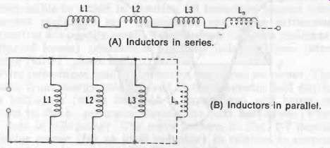
Fig. 8. Basic inductor circuits. (A) Inductors in series. (B) Inductors in parallel.

The property which has been under discussion up to this point is strictly termed self-inductance. When two inductors are so close physically that their fields overlap (that is, the coils are coupled), a second variety of inductance--mutual inductance (M)--comes into play. Interaction occurs because the first coil induces a counter emf into the second coil and vice versa (the effect differs from that resulting from the connection of two well-spaced inductors in series). When the two inductors are so tightly coupled (coefficient of coupling k = 1) that all the lines of force from one inductor link all the turns of the other, M is maximum, and when the two inductors are completely decoupled (that is, no flux from one interacts with the other) , M is zero.

4. NATURE OF INDUCTIVE REACTANCE

Fig. 9 shows the relationship between sinusoidal voltage and current for a pure inductance. Here, E, is the applied volt age, I is the resulting current, and E. is the counter emf. This counter voltage opposes the applied voltage, since-as is seen in Fig. 9--the two are out of phase with each other.

The counter voltage increases and the inductor current accordingly decreases as the frequency of the applied voltage increases, and vice versa. At a given frequency, the counter voltage increases and the inductor current therefore decreases as the inductance increases, and vice versa. An inductor there fore offers frequency-dependent opposition to the flow of alternating current. By means of calculus, it can be shown that this opposition is equal to wL. This opposition is termed inductive reactance, is measured in ohms, and is given by :

XL = wL= 2/ pi fL (1-12)

where, XL, is the inductive reactance in ohms,

L is the inductance in henrys,

f is the frequency in hertz,

w is 2 pi f,

pi is 3.1416.

The relations between current, voltage, and reactance are ex pressed in a form often called Ohm's law for ac:

XL = E, X E = IXL, and I =

(1-13)

where, XL is in ohms,

I is in amperes,

E is in volts.

From Equation 1-13, it is seen that an alternating current flowing in an inductive reactance produces a voltage drop IXL ; and, because of the phase of inductive reactance, this voltage leads the current by 90°.

Inductive reactance is a major factor in all LC circuits. It, like capacitive reactance (Section 1.6), is the property that imparts frequency sensitivity to these circuits. For a given inductance, doubling the frequency doubles the reactance, halving the frequency halves the reactance, and so on. Similarly, for a given frequency, halving the inductance, halves the reactance, doubling the inductance doubles the reactance, and so on. Appendix B gives the 1000-Hz reactance corresponding to ten inductances spaced in decade relationship from 1µH to 1000 H.

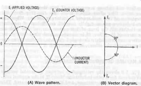
Fig. 9. Inductor current/voltage relationship. (A) Wave pattern. (B) Vector diagram.

5. NATURE OF CAPACITANCE

Capacitance (C or c) is the ability to store an electric charge.

It is somewhat analogous to the ability of a tank to store a quantity of fluid. Capacitance is measured in farads (F) ; but since this is an extremely large unit, submultiples of the farad generally are used (see Table 1-4). While capacitance exists between any two nearby conductors, it is primarily a property of capacitors. A simple practical capacitor consists of two identical metal plates or films separated by a dielectric (air, solid insulant, or liquid insulant), and its capacitance (C) is directly proportional to the area (A) of one plate and to the dielectric constant (k) of the dielectric, and is inversely proportional to the thickness (t) of the dielectric:

kA C = 4.45 t (1-14)

where, C is the capacitance in picofarads, k is the dielectric constant, A is the area of one plate in square inches, t is the thickness of the dielectric in inches.

Capacitors may be of the two-plate type or multiple-plate type. Both are manufactured in fixed and variable varieties and are offered in a wide range of capacitance and voltage ratings, shapes, and sizes. Numerous dielectrics (air, paper, oil, ceramic, mica, glass, plastic, etc.) are employed ; the higher the dielectric constant, the smaller the required area and thickness for a given capacitance. In addition to discrete capacitors, there are integrated capacitors which are processed into integrated circuits (ICs) . For special purposes, the internal capacitance of some other device-such as a vacuum tube, semiconductor diode or rectifier, or transistor-sometimes is employed instead of a capacitor per se.

Table 1-4. Units of Capacitance

When a dc voltage is applied to a capacitor, the latter be comes charged because energy then is stored in the electric field between the plates. When the voltage is disconnected, the capacitor retains the charge, the original voltage E appearing across the capacitor. If the capacitor were perfect, it would remain charged indefinitely. When an external circuit is connected across the charged capacitor, the capacitor discharges through the circuit and its voltage falls to zero. Thus, a cur rent flows into the capacitor to charge it, and out of the capacitor in the opposite direction to discharge it. No current can flow through the capacitor, because of the dielectric between the plates.

When a voltage (E) is applied to a given capacitor, the quantity of charge (Q) that the capacitor receives is directly proportional to the voltage and to the capacitance (C):

Q = CE (1-15)

where, Q is the quantity of charge in coulombs, C is the capacitance in farads, E is the voltage in volts.

When the voltage first is applied, a heavy current flows into the capacitor and the voltage across the capacitor is low.

This current diminishes with time while the capacitor voltage increases. When the capacitor becomes fully charged, the current ceases and the capacitor voltage then is equal to the charging voltage. Thus, the capacitor current leads the capacitor voltage. When an ac voltage is applied to a capacitor, charging current flows into the capacitor during one half-cycle, and discharging current flows out of the capacitor during the other half-cycle; so an alternating current flows in the circuit, but-again-not through the capacitor.

Because current leads voltage in a capacitor, the two are out of phase in a capacitor circuit. Pure capacitance would introduce a 90° phase shift in an ac circuit. Fig. 10 illustrates this 90°-leading phase feature. In both the wave plot (Fig. 10B) and the vector diagram (Fig. 10C), current and volt age are 90° out of step, with current leading at all points.

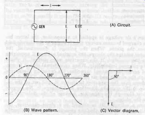
Fig. 10. Phase relationship: capacitance. (A) Circuit. (B) Wave pattern. (C) Vector diagram.

Examination of Fig. 10B shows that maximum capacitor current flows when the rate of change in voltage is maximum (i.e., when the ac voltage cycle is at zero) ; and, conversely, capacitor current is zero when the rate of change in voltage is zero (i.e., when the ac voltage cycle is at maximum). Here, I = C (de/dt). In this connection, see Section 1.1 for a discussion of rate of change. Because pure capacitance is impossible to attain in practice, all capacitors possess some inherent resistance and inductance, but these extraneous properties are usually tiny. Nevertheless, inherent resistance (internal losses) prevents a practical capacitor from introducing full 90° phase shift.

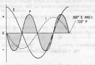
Fig. 11. Power in ideal capacitor.

Pure capacitance, unlike resistance (but like pure inductance), consumes no power. This is because energy stored in the electric field during charge is returned to the ac generator during discharge. The sine-wave pattern in Fig. 11 depicts capacitor power in relation to current and voltage (compare with Fig. 4, the wave pattern for resistor power, and Fig. 7, the wave pattern for inductor power). In a practical capacitor, the only power loss is that associated with the internal resistance of the capacitor, and this is small in a high grade capacitor.

When operating within their ratings, good-grade conventional capacitors undergo very little change in capacitance as a result of variations in voltage, temperature, or frequency.

Exceptions are voltage-variable capacitors (varactors), which are designed to be voltage sensitive, and compensating capacitors, which are designed to be temperature sensitive.

When capacitors are connected in series (Fig. 12A), the equivalent capacitance of the combination is :

(1-16)

When capacitors are connected in parallel (Fig. 12B), the total capacitance of the combination is :

Ct = C1 + C2 + C3 + …+ Cn (1-17)

If only two capacitors are connected in series, the equivalent capacitance of the combination is C = (C1C2)/ (C1 + C2).

If n capacitors, each having the same value C, are connected in parallel, the total capacitance of the combination Ct = nC.

If n capacitors, each having the same value C, are connected in series, the equivalent capacitance of the combination is Ceq = C/n.* [* For additional information on capacitance, see abc's of Capacitors written by William F. Mullin and published by Howard W. Sams & Co., Inc., Indianapolis, Indiana 46268.]

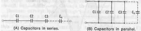
Fig. 12. Basic capacitor circuits. (A) Capacitors in series. (B) Capacitors in parallel.

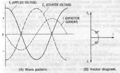
Fig. 13. Capacitor current/voltage relationship. (A) Wave pattern. (B) Vector diagram.

6. NATURE OF CAPACITIVE REACTANCE

Fig. 13 shows the relationship between the sinusoidal voltage and current for a pure capacitance. Here, Ei is the applied voltage, I is the resulting current, and E, the counter voltage. The latter is the voltage drop across the capacitor and is analogous to the counter emf developed by an inductor carrying alternating current. The counter voltage, Ec opposes the applied voltage, since-as is seen in Fig. 13--the two are out of phase with each other.

The counter voltage decreases and the capacitor current accordingly increases as the frequency of the applied voltage increases, and vice versa. For a given frequency, the counter voltage decreases and the capacitor current therefore in creases as the capacitance increases, and vice versa. A capacitor therefore offers frequency-dependent opposition to the flow of alternating current. By means of calculus, it can be developed that this opposition is equal to the reciprocal of wC. This opposition is termed capacitive reactance, is measured in ohms, and is given by :

1 1 X` a)C = 2 pi fC (1-18)

where,

X, is the capacitive reactance in ohms, C is the capacitance in farads, f is the frequency in hertz, w is 2 pi f, pi is 3.1416.

The relations between current, voltage, and reactance are ex pressed in a form often called Ohm's law for ac:

X, = T , E = IX,, and I = X, (1-19)

where, X, is in ohms, I is in amperes, E is in volts.

From Equation 1-19, it is seen that an alternating current flowing in a capacitive reactance produces a voltage drop IX, ; and because of the phase of capacitive reactance, this voltage lags the current by 90°.

Capacitive reactance is a major factor in all LC circuits used on ac. Like inductive reactance, it is the property that imparts frequency sensitivity to these circuits. For a given capacitance, doubling the frequency halves the reactance, quartering the frequency quadruples the reactance, and so on.

Similarly, for a given frequency, doubling the capacitance halves the reactance, and so on. Appendix C gives the 1000-Hz reactance for 126 common-stock capacitors between 5 pF and 5000 uF.

7. COMBINED REACTANCE IN LC CIRCUITS

When inductance and capacitance are operated in combination (series L and C, or parallel L and C), inductive reactance and capacitive reactance, being opposite in sign, oppose each other. Because of these phase relationships-illustrated by Figs. 6 and 10, respectively-the total reactance in the circuit is the difference between the two :

Xt = XL- XC (1-20) where, X XL, and X, are in the same units (ohms, kilohms, meg ohms, etc.).

Illustrative Example: A 16-henry inductor and 1-microfarad capacitor are operated in series at 400 hertz. Calculate the total reactance of this combination.

From Equation 1-12, XL = wL = 40,212 ohms; and from Equation 1 18, X, = 1/c0C = 398 ohms.

From Equation 1-20, X, = 40,212- 398 = 39,814 ohms.

8. RESONANCE

When inductance and capacitance are operated in combination, inductive reactance XL is dominant at low frequencies and capacitive reactance X, is dominant at high frequencies.

At a sufficiently low frequency where XL >> X, the phase angle (0) of the circuit will reach a maximum value of +90°; and at a sufficiently high frequency where X, >> XL, the phase angle will reach a maximum value of-90°. At a frequency somewhere between these two extremes, which depends upon the L and C values, the total reactance, X,, of the circuit is zero (since at that point X, = XL- X, = 0), and the phase angle is zero. The frequency at which this situation occurs is the resonant frequency (fr) of that particular LC combination :

1 f'-

2 pi V LC where, f is in hertz, L is in henrys, C is in farads, IT is 3.1416.

(1-21)

Illustrative Example: Calculate the resonant frequency, in kHz, of a circuit containing 1 mH and 250 pF.

Here, 1 mH = 0.001 H, and 250 pF = 2.5 x 10^-10 F.

From Equation 1-21 f, = 1/(6.2832 V0.001 x 2.5 x 10-10) 1/(6.2832 V2.5 x 10^-13) = 1/(6.2832 x 5 x 10-7) = 1/ (3.1416 x 10^-6) = 318,309 Hz = 318.3 kHz.

9. FIGURE OF MERIT

Since practical inductors and capacitors have inherent resistance, they can function efficiently as reactors only when this resistance is low. The ratio of reactance to resistance therefore is an indicator of this effectiveness and is termed figure of merit, symbolized by the letter Q. Thereby, Q = XL/R = Xe/R, where X1 X and R are in ohms. The resistance acts for the most part in series with the inductor or capacitor.

For the inductor :

(1-22)

where, f is in hertz, L is in henrys, R is in ohms.

For the capacitor :

(1-23)

where, f is in hertz, C is in farads, R is in ohms.

The series resistance of a capacitor is virtually impossible to measure directly, and usually is determined by calculation from Q measurements (R = Xc/Q). The resistance of an inductor at dc and low frequencies is quite entirely the dc resistance of the wire in the coil. While at low frequencies, the resistance component has the same value as the easily measured dc resistance, at very high frequencies the resistance is a combination of de resistance and all in-phase opposition arising from skin effect, influence of dielectrics in the magnetic field, and influence of shielding.

10. NATURE OF PRACTICAL INDUCTOR

It was mentioned earlier that a practical inductor, unlike the ideal pure inductance, has inherent resistance. It also has internal capacitance (termed distributed capacitance).

These stray components are shown in relationship to the inductance, in Fig. 14. The resistance is occasioned by the wire with which the coil is wound and, at very high frequencies, also by skin effect and other factors. It is minimized by using thick wire or, especially at radio frequencies, braided wire. The shunting capacitance results from capacitor effect between adjacent turns and between layers of turns, and it is minimized by spacing the turns and by special styles of winding in which the turns are crisscrossed to destroy their adjacency.

Internal R and Cd combine with L to make an inductor an impedance, rather than a simple reactor, and in many applications it must be dealt with as such. The detrimental effect of resistance has already been pointed out in the discussion of Q in Section 1.9. Depending upon frequency, the distributed capacitance can limit the range over which a given inductor can resonate with a selected external capacitor.

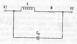
Fig. 14. Equivalent circuit of practical inductor.

11. PURE L AND C IN COMBINATION

For the moment, we will neglect the resistance that is al ways present, in however small amount, in LC circuits and will consider the effect of pure inductance in combination with pure capacitance, the ideal LC circuit. The effect of resistance will be saved for separate discussion in Section 1.12.

Inductance and Capacitance in Series

In the series LC circuit (see Fig. 15A), the total reactance is equal to XL- X, and is zero at resonance. As the frequency is varied, the phase angle increases to +90° at the frequency at which XL >> Xe, and increases to-90° at the frequency at which X, >> XL. The angle is zero at resonance, where XL = X,.

Inductance and Capacitance in Parallel

In the parallel LC circuit (see Fig. 15B), the total reactance is equal to L [C (XL- X,)] , and is infinite at resonance.

Fig. 15. Basic combinations of pure inductance and capacitance. (A) L and C in series. (B) L and C in parallel.

As the frequency is varied over a sufficient range, the phase angle is zero at resonance, and it increases to +90° when XL >> X, and increases to-90° when X, >> XL.

As the losses in inductors and capacitors are reduced, performance approaches that of the ideal inductor and capacitor.

Indeed, when extremely high-Q inductors and capacitors are available for a given application, their remaining resistance sometimes is so small as to be ignored so that circuit design may proceed as if pure inductance and capacitance were being used. In most instances, however, the resistive component cannot be ignored, and its influence is treated in the next section.

12. PRACTICAL L AND C IN COMBINATION

Since the inherent resistance in an LC circuit usually can not be neglected, it must be dealt with in most analyses and design of LC circuits. At resonance, reactance disappears, but in a practical LC circuit resistance does not. An LC circuit thus is most often an LCR circuit ; and when resistance enters, we must talk about impedance, not just simple reactance. Impedance Z_ohms = _/ [Rohms^2 X_ohms^2].

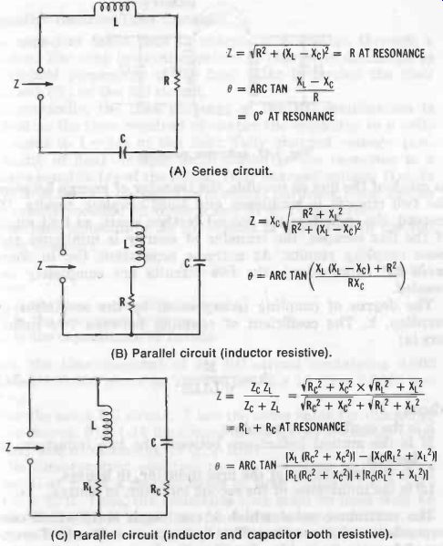
Fig. 16 shows the basic LCR arrangements.

Series Circuit

See Fig. 16A. In this circuit, resistance R may be due entirely to inductor L or it may be the combined resistance of inductor and capacitor. In any event, it is shown as the single series resistance. Note from the impedance equation in Fig. 16A that the impedance of this circuit is the simple vector sum of resistance (R) and total reactance (XL- Xc). The equation for the phase angle also is relatively simple, being the arc tangent of the total reactance to the resistance. Note also that at resonance, the impedance is R. the value of the circuit resistance (the reactance having disappeared).

Parallel Circuit No. 1

See Fig. 16B. In this circuit, only the inductor has significant resistance. This is often the case, where the capacitor has such a high Q, compared with that of the inductor, that entering the tiny capacitor resistance into the calculations will needlessly complicate them and contribute little to the final result. Note that the impedance of this circuit is more complicated than that of Fig. 16A.

Parallel Circuit No. 2

See Fig. 16C. While the condition shown in Fig. 16B is often the case in practice, it is not always so. There are many instances in which the inductor and capacitor each have significant resistance (R_L and R_C). Note here that the impedance equation and the phase-angle equation are the most complex of all.

Fig. 16. Basic LCR circuits. (A) Series circuit. (B) Parallel circuit (inductor resistive). (C) Parallel circuit (inductor and capacitor both resistive).

13. INDUCTIVE COUPLING

Two inductors are coupled when the magnetic field of one cuts the turns of the other so that energy is transmitted from one to the other or, conversely, so that energy is absorbed by one from the other. Thus, in Fig. 17, the magnetic flux resulting from current flow in the primary L1C1 circuit induces a voltage across inductor L2, and this causes a current to flow in the secondary, L2C2, circuit. If the inductors are placed as close together as possible and correctly oriented, so as to utilize as much of the flux as possible, the transfer of energy between the two circuits is maximum and tight coupling results. If, instead, the inductors are spaced farther apart, so that much of the flux escapes, the transfer of energy is minimum and loose coupling results. At extreme separation (or in some cases 90° orientation), the two circuits are completely decoupled.

The degree of coupling is expressed by the coefficient of coupling, k. The coefficient of coupling between two inductors is :

k = V L1L2

(1-24)

where, k is the coefficient of coupling, M is the mutual inductance between the two inductors, in henrys, L1 is the inductance of the first inductor, in henrys, L2 is the inductance of the second inductor, in henrys.

The maximum value which k can reach is 1, which corresponds to 100% coupling. This figure can result only if every line of force in the linking flux is utilized.

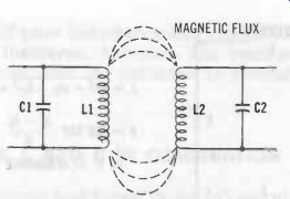
Fig. 17. Inductive coupling.

14. TIME CONSTANT

Capacitors and inductors both are subject to delayed response when they are operated in series with resistors. When a capacitor is charged through a resistor, time is required for the charge to be completed, i.e., for the voltage across the capacitor to equal the source voltage. Similarly, when a voltage is applied to an inductor in series with a resistor, time is required for the current flowing through the inductor to stabilize, i.e., to rise to its final, steady value.

Capacitor-Resistor Time Constant

A capacitor takes time to charge or discharge through a resistor. The time interval required to charge or discharge to a standard percentage of the final value is termed the time constant (T) of the RC circuit.

Numerically, the time constant of the RC combination is defined as the time required to charge the capacitor to a volt age equal to 1- 1/E of the final, fully charged voltage (i.e., to 63.2% of final voltage) or to discharge the capacitor to a voltage equal to 1/E of the initial, fully charged voltage (i.e., to 36.79% of initial voltage).

For practical purposes, these figures are usually rounded off to 63% and 37%, respectively.

The time constant of an RC circuit is calculated in the following manner :

T = RC (1-25)

Where

T is the time constant in seconds,

R is the resistance in ohms,

C is the capacitance in farads.

Thus, the time constant of an RC circuit containing 0.002 uF and 100,000 ohms is T = 100,000 (2 x 10^-9) = 0.0002 s = 0.2 ms.

For the same RC circuit, T has the same value for discharge as for charge. Fig. 18 illustrates the progress of charge (Fig. 18A) and of discharge (Fig. 18B).

The time-constant equation can be rewritten to determine either R or C for a desired value of time constant : R = T /C, and C = T/R. Thus, the resistance that must be used with an available 0.005-µF capacitor for a 1-microsecond time constant = T/C = (1 x 10^-6)/(5 x 10^-9) = 200 ohms. Similarly, the capacitance required with a 50,000-ohm resistor for a time constant of 48 seconds = T/R = 48/50,000 = 960 µF.

Appendix D gives the time constants of a number of common RC combinations ranging from 0.0001 microfarad with 1 ohm to 1000 microfarads with 10 megohms.

Inductor-Resistor Time Constant

After application of voltage, a time interval is required for current to reach a maximum in an inductor operated in series with a resistor. Numerically, the inductor-resistor time constant is defined as the time required for the current flowing through the inductor to reach a value equal to 1- 1/E of its final, steady value (i.e., to 63% of final value).

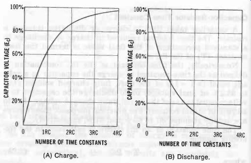
Fig. 18. RC time constant. (A) Charge. (B) Discharge.

The time constant of an LR circuit is calculated in the following manner :

T = R (1-26)

where, T is the time constant in seconds, L is the inductance in henrys, R is the resistance in ohms (including internal resistance of the inductor).

Thus, the time constant of an LR circuit containing a 20-henry inductor (internal resistance, 900 ohms) in series with 5000 ohms is T = 20/ (900 + 5000) = 20/5900 = 0.0034 s = 3.4 ms.

Fig. 19 illustrates the progress of current growth in an LR circuit.

The time-constant equation can be rewritten to determine either R or L for a desired value of time constant : L = RT, and R = L/ T. Thus, the total resistance (external resistance plus inductor-coil resistance) that must be used with an available 8-henry inductor for a 10-millisecond time constant is R = L/T = 8/0.01 = 800 ohms. Similarly, the inductance required with a 27-ohm resistor for a time constant of 2 seconds is L RT = 27 (2) = 54 H.

Appendix E gives the time constants of a number of inductor-resistor combinations ranging from 100 microhenrys with 1 ohm to 1000 henrys with 10 megohms.

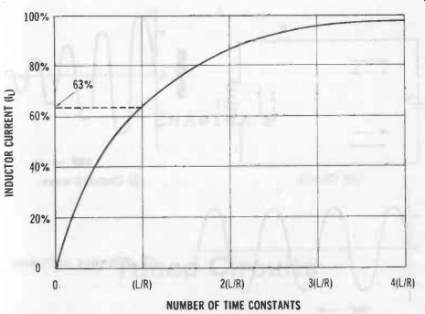
Fig. 19. L/R time constant

15. OSCILLATIONS IN LC CIRCUIT

If a capacitor is charged (say, with its upper plate positive, as shown by the solid + in Fig. 20A) and then has an inductor, L, connected across it, the capacitor will proceed to discharge through the inductor, the electrons on the negative plate passing through the inductor, as shown by the solid arrow. This action, transferring the electrons from one plate to the other, recharges the capacitor to the opposite polarity, and the current causes a magnetic field to expand about the inductor. But when the capacitor becomes fully recharged, the current ceases and the magnetic field collapses. The collapsing field then induces a voltage of opposite polarity at the inductor terminals, and this voltage discharges the capacitor, causing a current to flow in the opposite direction (see dotted arrow) and the original polarity of the capacitor to be re stored. The action then repeats itself periodically as the capacitor charges in first one direction and then the other, and the inductor field alternately expands and collapses. An alternating current thus flows in the circuit.

Once started, this action would continue forever, but the circuit has internal resistance (see dotted R in Fig. 20A) which absorbs energy and eventually stifles the oscillations.

Thus, when a single impulse starts the chain of events, the amplitude of each cycle, like the swing of a pendulum given only a single push, will be lower than that of the preceding one (see Fig. 20B) until the oscillations finally die out. A damped wave is the result. The higher its Q, the longer the circuit will "ring" in response to a single exciting pulse.

In a complete practical oscillator circuit, a tube or transistor supplies just enough energy in the proper phase to overcome the losses of the LC circuit, and this sustains the oscillations at constant amplitude to correct the damping shown in Fig. 20B. Thus, the LC circuit actually is the oscillating medium, but its action must be sustained, like that of a pendulum or flywheel, by little pushes of energy from a tube or transistor.

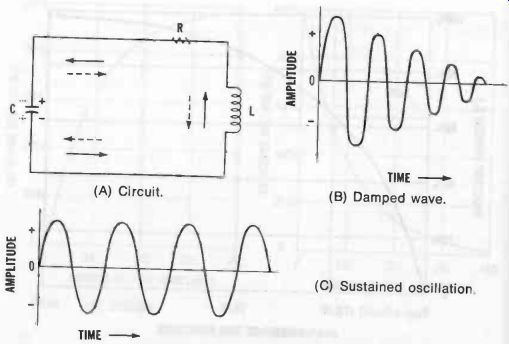
Fig. 20. Oscillations in LC circuit.

16. RANGE OF APPLICATION OF LC CIRCUITS

Both fixed and variable LC circuits enjoy a wide range of applications. A few of the common devices in which these circuits provide the basis of operation are of and rf tuning networks, tuned transformers, filters (both signal and power supply), voltage regulators, discriminators, ratio detectors, wavetraps, and test instruments (bridges, comparators, wave meters, null devices, etc.).