LC Circuits--TUNED CIRCUITS

The first business of the LC circuit was the tuning of radio equipment; and, after more than three-quarters of a century, this simple circuit is still doing that job-with the added function of tuning television. It is doing other jobs, both at radio and audio frequencies; however, even in its most sophisticated modern applications far removed from simple tuning, the LC circuit still is, at core, providing selectivity.

Advancing the explanation introduced in Section 1, the present Section describes the LC circuit qua tuner, and presents a number of its applications in that function. There are many more, of course, than can be included in this Section. But even this brief survey should highlight the versatility of this simple combination of passive components.

The reader should return often to Sections 1.11 and 1.12 in Section 1 if he needs to strengthen his understanding of the material in the present Section.

1. SERIES-RESONANT CIRCUIT

Fig. 1A shows a series-resonant circuit, so called because in this arrangement, generator GEN, inductance L, capacitance C, and internal resistance R are connected in series.

The resonant frequency (fr) of the circuit depends upon the L and C values in the following relationship:

f_r=1/ 2 pi √LC

(2-1)

where, fr is the resonant frequency in hertz, L is the inductance in henrys, C is the capacitance in farads, pi is 3.1416.

Illustrative Example: Calculate the resonant frequency in megahertz of a series-resonant circuit containing an inductance of 50 /LH and a capacitance of 75 pF.

Here, L = 5 x 10^-5 H, and C = 7.5 x 10^-11 F.

From Equation 2-1, fr = 1/6.283 V5 X 10-5 (7.5 X 10^-11) = 1/6.283 43.75 x 10^-15 = 1/6.283 (6.124 x 10^-8) = 1/3.845 x 10^-7 = 259,895 Hz = 2.599 MHz.

When the inductance and capacitance are fixed, the circuit has a single resonant frequency. Often, however, either L or C or both are variable, and the circuit can be adjusted over a range of resonant frequencies.

In Fig. 1A, the ac generator delivers a constant voltage (E), forcing a current (I) through the circuit. At resonance, the inductive reactance and the capacitive reactance cancel each other, leaving only the internal resistance to determine the current. Maximum current therefore flows at resonance.

(This is another way of saying that the impedance of the series-resonant tuner is lowest at resonance.) This performance is shown in Fig. 1B. Note from these curves that the sharpest response and greatest height (highest selectivity) are obtained when resistance is lowest, and the broadest response and lowest height when resistance is highest. High selectivity (sharp tuning) corresponds to high Q, and vice versa.

The response in Fig. 1B may be obtained by either holding L and C constant and varying the generator frequency, or by holding the frequency constant and varying L or C. It is interesting to note that to the generator the series-resonant circuit looks like an inductor (in series with the internal resistance of the latter) at frequencies above resonance, like a capacitor (in series with the internal resistance) at frequencies below resonance, and like a resistor (the internal resistance) at resonance.

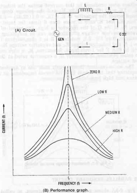
Fig. 1. Series-resonant circuit. (A) Circuit. (B) Performance graph.

An important effect observed in the series-resonant circuit is resonant voltage step-up. This means that at resonance, the voltage (E_L) across the inductor and the voltage (E_C) across the capacitor each will be higher than the generator voltage.

However, this phenomenon does not violate Kirchhoff's second law, for E_L, and Ec are 180° out of phase with each other, and the sum of the voltage drops around the circuit equals the supply voltage. Fig. 2 illustrates this effect. In this arrangement, the input voltage (Ei) is 1 V at 1000 Hz, the resonant frequency of the LC combination. Thus, XL = Xc = 62.83 ohms, and internal resistance R = 10 ohms. Since the total reactance at resonance is zero, the current flowing in the circuit depends entirely upon the resistance; i.e., I = E/R = 1/10 = 0.1 A, and this current flows through the inductor and capacitor. The voltage drop produced by this current across the inductor is EL = I X_L = 0.1 (62.83) = 6.28 V ; and the voltage drop produced across the capacitor is E, = IX, = 0.1 (62.83) = 6.28 V.

Thus, Er, and Ec each is more than 6 times the input volt age, E. If the Q of the inductor is high, the extent of this transformerless voltage amplification can be surprising. For instance, if in Fig. 2, resistance R is 1 ohm, current I will be 1 A, and inductor voltage EL and capacitor voltage E, each will be 62.8 V for 1-volt input. Sometimes, Ec is high enough to cause puncture or flashover in a capacitor rated at the in put voltage.

The series-resonant tuner circuit finds use in applications requiring that the circuit have its lowest impedance at resonance and high impedance off resonance.

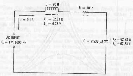
Fig. 2. Resonant voltage step-up circuit.

2. PARALLEL-RESONANT CIRCUIT

Fig. 3A shows a parallel-resonant circuit, so called be cause in this arrangement, generator GEN, inductance L, and capacitance C are connected in parallel. The internal resistance of this circuit is mainly in the inductor leg, as shown by R. As in the series-resonant circuit, the resonant frequency (fr) of the parallel-resonant circuit depends upon the L and C values, in the same relationship. Therefore, Equation 2-1 applies also to the parallel circuit.

When the inductance and capacitance are fixed, the circuit has a single resonant frequency.

Often, however, either L or C or both are variable, and the circuit can be adjusted over a range of resonant frequencies.

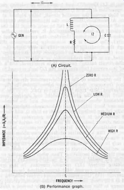
Fig. 3. Parallel-resonant circuit. (A) Circuit. (B) Performance graph.

In Fig. 3A, the ac generator delivers a constant voltage (E), forcing a current (I1) through the parallel circuit.

Within the circuit, this current divides into two components (IL in the inductive leg and I,, in the capacitive leg-neither shown) which are out of phase with each other. The net result of these two currents is current 12 flowing within the LC circuit as a result of charge and discharge of the capacitor through the inductor (See Section 1.15 in Section 1, "Oscillations in LC Circuit") and termed the circulating current.

The opposition of IL and L. to each other causes the impedance to be high across the parallel circuit, being highest at resonance. At resonance, therefore, the input current, I1, is lower than off resonance (it would fall to zero, except that the parallel circuit has internal resistance, R, remaining after cancellation of the reactance; therefore, the current cannot reach infinity). The result is the interesting phenomenon that al though the circulating current (I2) is very high, the input current (I1) is very low at resonance. This mechanism is of ten used, as in radio transmitters, as a sensitive indicator of parallel-circuit tuning: current Il is monitored, and a sharp dip of this current indicates that the LC tank is tuned to resonance.

If the impedance of the parallel-resonant circuit is plotted against frequency, the response curves shown in Fig. 3B are obtained. Note from these curves that, as in the series-resonant circuit, the greatest height and sharpest response are obtained when resistance is lowest, and the broadest response and least height when resistance is highest. High selectivity (sharp tuning) corresponds to high Q, and vice versa.

It is interesting to note that to the generator the parallel-resonant circuit looks like an inductor (in series with the internal resistance of the latter) at frequencies below resonance, and like a capacitor at frequencies above resonance.

As was explained in Section 1.15 in Section 1, it is necessary only to supply enough additional energy in proper phase to an oscillating LC circuit to overcome circuit losses, in order to keep the circuit oscillating. Thus, when a transistor or tube supplies the needed pulses to a parallel-resonant circuit, the circulating current (I2) remains constant. In this way, a large circulating current (I2) is maintained for a small in put current (I1) , the parallel-resonant circuit behaving some what as a flywheel. Because the parallel-resonant circuit stores ac energy in this manner, it is frequently termed a tank circuit, or just a tank.

The parallel-resonant tuner circuit finds use in applications requiring that the tuned circuit have its highest impedance at resonance and low impedance at frequencies off resonance.

3. RESONANT-CIRCUIT CONSTANTS

The resonant frequency of a tuned circuit can be determined from Equation 2-1 when L and C both are known. In some in- stances, either L or C will be unknown, and the equation may be rewritten for that component :

Inductance unknown 1 L =

4 pi^2f^2 C (2-2)

where, L is the unknown inductance in henrys, C is the available capacitance in farads, f is the desired resonant frequency in hertz, 471-2 is 39.5.

Illustrative Example: An accurate 0.0047uF capacitor is available. What value of inductance (in mH) will resonate this capacitance to a frequency of 1 MHz? Here, C = 4.7 x 10^-9F, and f = 1 X 10^6 Hz.

From Equation 2-2, L = 1/(39.5 (1 x 106)2 4.7 x 10^-9) = 1/(39.5 (1 x 10^12) 4.7 x 10^-9) = 1/30.5 (4.7 x 10^3) = 1/185,650 = 5.39 X 10^-6H = 0.00539 mH.

Capacitance unknown

1 4 pi 2 f^2 L (2-3)

where, C is the unknown capacitance in farads, L is the available inductance in henrys, f is the desired resonant frequency in hertz, 4r^2 is 39.5.

Illustrative Example: An 8.5-henry inductor is available. What value of capacitance (in AF) will resonate this inductance to a frequency of 120 Hz?

From Equation 2-3, C = 1/(39.5(1202) 8.5) = 1/(39.5(14,400)8.5) = 1/4,834,800 = 2.068 x 10^-7F = 0.2068 µF. (This value can be made up by connecting one 0.2- and one 0.0068-µF capacitor in parallel.)

Appendix F gives the resonant frequency of a number of combinations from 1 microhenry and 10 picofarads to 1000 henrys and 1000 microfarads, and applies both to series-resonant and parallel-resonant circuits.

4. SELECTIVITY

Selectivity is the sharpness of response of a tuned circuit. It expresses the ability of a pass-type circuit to select a signal of desired frequency and suppress all others, or the ability of a reject-type circuit to suppress a signal of undesired frequency and pass all others.

Fig. 4 shows a selectivity curve. A plot of this type is obtained by applying a constant input voltage to the tuned circuit and tuning the generator above and below resonance.

The resonant point is indicated by peak upswing (as in Fig. 4) of voltage or current in a pass-type circuit, or by maxi mum dip (where Fig. 4 would be inverted) in a reject-type circuit. Voltage, current, or arbitrary units may be plotted along the vertical axis, frequency along the horizontal. The 100% point in this illustration merely designates maximum height (current, voltage, etc.) of the curve under study. The selectivity curve consists of its tip (called the nose) and its sides (called the skirts). Depending upon the characteristics of the circuit, some curves are blunt nosed and others are pointed.

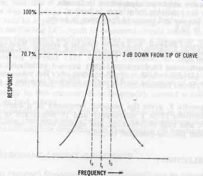
Fig. 4. Selectivity curve.

It is apparent from the width of the curve that a practical tuned circuit is not completely single-frequency responsive, but operates over a narrow band of frequencies. The more selective the circuit, the narrower this band. At any point, the bandwidth of the curve-in Hz, kHz, or MHz-is the width at a selected point. This point is usually stated. Thus, in Fig. 4, the bandwidth at 70.7% of maximum rise (i.e., 3 dB down from maximum) is equal to the frequency difference fb- fa.

A sharply tuned circuit has good skirt selectivity (the ratio of the bandwidth at one point, say 3 dB, to that at another point, say 60 dB).

5. CIRCUIT Q

It is clear from the resonance curves shown earlier--Figs. 1B and 3B-that high selectivity is the result of high Q, and vice versa. This permits the value of circuit Q to be approximated closely by finding the ratio of resonant frequency (fr) to bandwidth (BW). This is done in the laboratory by inductively coupling the tuned circuit loosely to a constant-output-voltage signal generator, tuning the generator above and below the resonant frequency, noting the current or voltage response, and calculating Q as the ratio of resonant frequency to bandwidth at the -3-dB point: (1) With reference to Fig. 4, tune the generator to the resonant frequency (fr) and note the value of circuit voltage or current at this point. (2) Detune the generator below resonance to the frequency (f.) at which the circuit voltage or current falls to 70.7% of its resonant value. This is 3 dB below resonant voltage or cur rent. (3) Next, detune the generator above resonance to the frequency (fb) at which the circuit voltage or current falls again to 70.7%. (4)

Then, calculate Q:

f f,. f BW If fb- fa (2-4) where, all frequencies (f's) are in the same unit (Hz, kHz, or MHz).

---------------

Illustrative Example: A certain tuned circuit is tested with a signal generator and high-input-impedance electronic ac voltmeter. The resonant frequency (fr) is found to be 2.5 MHz, and the generator out put voltage is adjusted for exactly 100 mV across the inductor. The generator then is detuned below resonance to the frequency at which the inductor voltage falls to 71 mV (approximately 70.7% of resonant voltage), and this frequency (ft) is 2.3 MHz. Next, the generator is detuned above resonance to the frequency at which the inductor voltage again falls to 71 mV, and this frequency (fb) is 2.7 MHz. Calculate the Q of this circuit.

From Equation 2-4, Q = 2.5 2.5 6.25.

7- 2.3- 0.4

--------------

Drawing energy from a tuned circuit ("loading" the circuit) tends to reduce the selectivity and Q, because the drain constitutes a loss which resembles the equivalent resistance reflected back into the tuned circuit. This action is reduced by lightly loading the circuit whenever possible.

6. COUPLED RESONANT CIRCUITS

When identical resonant circuits are cascaded, the selectivity of the combination is higher than that of any one of the circuits. Thus, the tuning of an electronic equipment is sharpened (bandwidth reduced) by cascading several LC circuits for ganged tuning. Often, an amplifying device-tube, transistor, or IC-operates between successive LC circuits, but in many instances the resonant circuits are simply capacitance coupled, as shown in Fig. 5A. Paradoxically, coupled resonant circuits are used also for the opposite purpose : to broaden tuning under controlled conditions. For example, one of two circuits is resonated at a higher frequency than the other, and the two circuits together offer a wider pass-band (broader-nosed curve) than is afforded by one circuit alone.

In Fig. 5A, the resonant circuits (L1, C1, L2, C3, L3 C5) are spaced far enough apart to eliminate mutual inductance between them, and the coupling of energy from one to the other is entirely via capacitors C2 and C4. Although this circuit narrows the passband, the resonant voltage may be reduced across successive tanks, depending upon the reactance of C2 and C4.

Inductive coupling (also called transformer coupling) takes many forms. In every case, however, the coupling is accomplished by means of the mutual inductance between the two inductors. The input is called the primary circuit, and the output the secondary.

Fig. 5 (B to E) shows several examples. In Fig. 5B, the input and output circuit each is series resonant; in Fig. 2 5C, input is series resonant and output is parallel resonant; in Fig. 5D, input is parallel resonant and output is series resonant ; and in Fig. 5E, input and output each is parallel resonant. Series resonance is used for low-impedance input or output, and parallel resonance for high-impedance input or output. The parallel-in/parallel-out circuit is a familiar one, being the type found in rf, if, and detector transformers and in tuned audio transformers.

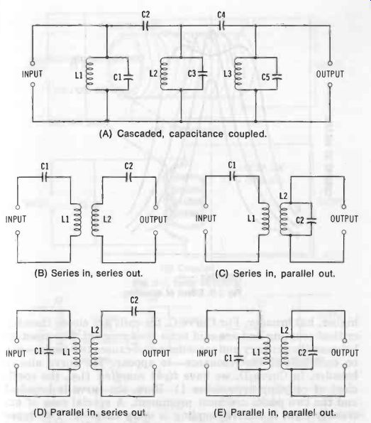
Fig. 5. Coupled resonant circuits. (A) Cascaded, capacitance coupled. (B) Series in, series out. (C) Series in, parallel out. (D) Parallel in, series out. (E) Parallel in, parallel out.

In inductively coupled circuits, the degree of coupling greatly influences the selectivity of the circuit. The secondary loads the primary, and the primary loads the secondary; and this mutual action increases as the coupling grows tighter, tending to broaden the response. Fig. 6 shows the differences which result when a constant voltage is applied to the tuned circuit and the coupling is changed. The primary and secondary are tuned to the same frequency. In this illustration, Curve A-the sharpest-corresponds to loose coupling (coils well separated). Curve B shows critical coupling, the condition in which maximum energy is drawn from the tuned circuit. Here, the coils are more closely spaced, so the peak is higher, but broader. For Curve C, the coils are closer than for critical coupling and are said to be close coupled. The reaction between the primary and secondary now causes two peaks-one on each side of the resonance-to appear. The curve also is broader. In Curve D, we have tight coupling (i.e., the coefficient of coupling approaches 1). Here, the curve is broadest and the two peaks are most prominent. A special case of extremely tight inductive coupling is unity coupling. Two types are shown in Fig. 7. As shown, the turns of secondary coil L2 (dotted line) are inter-wound with those of primary coil L1 (solid line). In Fig. 7B, primary coil L1 is wound with hollow tubing, and secondary coil L2 (dotted line) consists of an insulated wire threaded through this tubing coil. In unity coupling, mutual inductance M is so high that a single capacitor, C1, tunes both L1 and L2.

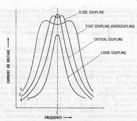
Fig. 6. Effect of coupling.

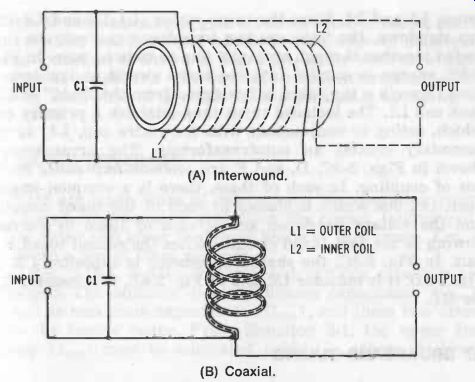
Fig. 7. Unity coupling. (A) Inter-wound. (B) Coaxial.

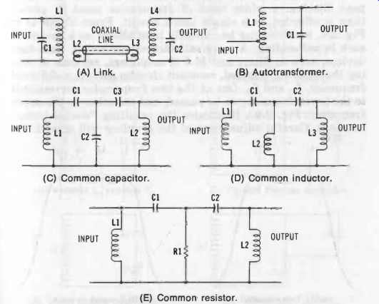
Fig. 8. Miscellaneous coupling methods. (A) Link. (B) Autotransformer. (C) Common capacitor. (D) Common inductor. (E) Common resistor.

Fig. 8 shows several additional methods of coupling. Fig. 8A shows the familiar link coupling, which is widely used in radio transmitters and other equipment in which the two tuned circuits must be spaced far apart. The "links" consist of coils L2 and L3, each usually 1 to 3 turns wound around the "cold" end of the tank coil (LI., L4). They provide the inductive coupling which is impossible to obtain directly be- tween L1 and L4. Since the turns ratios (L1:L2 and L4 :L3) are stepdown, the links are low impedance and may be connected together through a coaxial line or twisted pair. In Fig. 8B, energy is coupled into the tuned circuit at low impedance through a tap taken a few turns from the "cold" end of tank coil L1. The included turns thus establish a primary coil which, acting in conjunction with the entire coil, L1, as the secondary creates an autotransformer. The arrangements shown in Figs. 2-8C, D, and E are common-impedance methods of coupling. In each of these, there is a common impedance, i.e., one which is shared by each of the tuned circuits, and the voltage developed across each of these by current flowing in the first tuned circuit excites the second tuned circuit. In Fig. 8C, the shared impedance is capacitor C2, in Fig. 8D, it is inductor L2, and in Fig. 8E, it is resistor R1.

Fig. 9. Broadband response. (A) Two circuits. (B) Several circuits.

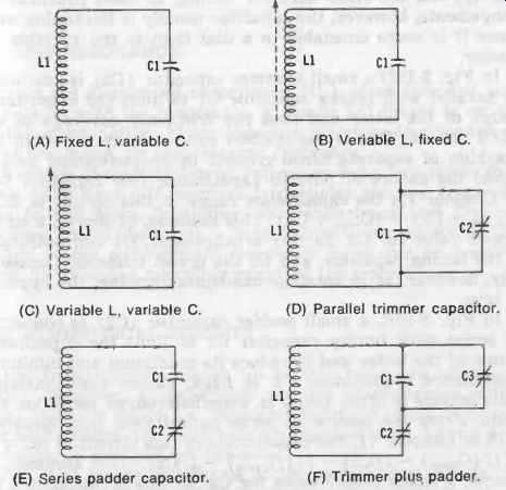
Fig. 10. Variable tuning arrangements. (A) Fixed L, variable C. (B) Variable L, fixed C. (C) Variable L, variable C. (D) Parallel trimmer capacitor. (E) Series padder capacitor. (F) Trimmer plus padder.

7. BROADBAND TUNING

In some applications, such as high-fidelity radio and band pass filtering, a wider band of frequencies must be passed than is afforded by a single tuned circuit. From Curve D in Fig. 6, overcoupling has already been shown as a means of such broad-banding. A more satisfactory method in fixed-tune devices, such as filters and hi-fi if amplifiers, consists of tuning the separate, coupled, resonant circuits each to a different frequency, fr., and fr.. One of the two frequencies corresponds to the lower frequency to be passed, and the other to the upper frequency. Fig. 9A illustrates the resulting "double-hump" response. Careful adjustment of the coupling will smooth the humps to some extent and give a flatter, broader-nosed, curve.

For a wider band, several tuned circuits may be employed, being connected as shown in Fig. 5A, either with or without interposed amplifiers. The separate resonant frequencies result in somewhat of a ripple in the passband, as shown in Fig. 9B.

8. RANGE COVERAGE

There are many ways of determining the operating range of a tuned circuit and of presetting the circuit (aligning it) at the upper and lower frequency limits of that range. Fig. 10 shows a few of these methods.

In Fig. 10A, a fixed inductor and variable capacitor are employed. The capacitor has a minimum capacitance (C_min) , as well as maximum capacitance (Cmax), and these two deter mine the tuning range. From Equation 2-1, the upper frequency (fmax) must be calculated, using C_min; then, the lower frequency (f_min) must be calculated, using C_max. The tuning range, Af, then is f-max faun, and the frequency coverage is f_min + delta_f.

In Fig. 10B, inductor L1 is variable, and capacitor C1 is fixed. Inductance may be varied in several ways. In low-power rf applications and in some of applications, the inductance is adjusted by means of a slug, as indicated in the schematic ; in transmitters and industrial oscillators, the coil may have a series of taps or a turns-contacting slider for this variation, or the coil can be a variometer (a device consisting of two coils in series, one rotatable inside the other). In Fig. 2 10B, the coil has a minimum inductance (L), as well as a maximum inductance (Lmax) which will determine the tuning range. From Equation 2-1, the upper frequency (fmax) must be calculated, using L,, ; then, the lower frequency (f,,) must be calculated, using Lm. The tuning range, Af, then is fmax fmin, and the frequency coverage is fd + Af.

In Fig. 10C, inductance and capacitance both are variable.

Either one may be used to set the circuit to a range-limit frequency, and the other used for tuning. In most practical arrangements, however, the capacitor usually is the tuning unit, since it is more amenable to a dial than is the variable inductor.

In Fig. 10D a small trimmer capacitor (C2) is connected in parallel with tuning capacitor C1 to limit the capacitance range of the latter and thus the frequency coverage of the L1C1 circuit. This is the method commonly employed in the tracking of separate tuned circuits in ganged-tuning setups.

From the nature of parallel capacitance (see Equation 1-17 in Section 1), the capacitance range in this circuit is AC = (C1max C2) - (C1min, + C2).

This assumes, of course, a single preset value for C2. In this arrangement, C1 conventionally is the tuning capacitor, and C2 the preset trimmer. Occasion ally, however, as in amateur bandspread tuning, the opposite is true.

In Fig. 10E, a small padder capacitor (C2) is connected in series with tuning capacitor C1 to limit the capacitance range of the latter and to reduce its maximum and minimum capacitance. Sometimes, C2 is fixed, rather than variable.

This scheme is often found in superheterodyne oscillator circuits. From the nature of series capacitance (see Equation 1-16 in Section 1), the capacitance in this circuit is AC = 1/ {(1/ (C1.)- 1/C2]- [(1/C1min)- 1/C2]. This assumes, of course, a single preset value for C2. In this arrangement, C1 conventionally is the tuning capacitor, and C2 the preset padder. Occasionally, however, as in amateur bandspread tuning, the opposite is true.

In Fig. 10F, a combination of the two preceding methods is employed. Both a series padder (C2) and parallel trimmer (C3) are employed for close pruning of the capacitance range of main tuning capacitor C1.

In each of the foregoing examples, the distributed capacitance (Cd) of the inductor has been neglected, since it is usually small compared to the capacitance of the tuning, trimmer, and padder capacitances in the circuit. But, in some radio-frequency circuits--especially where very small tuning capacitances are employed-distributed capacitance cannot be ignored. For example, a popular 10-mH inductor has a distributed capacitance of 4 pF. If this coil is used in a tuned circuit, such as Fig. 10A, with a 100-pF variable capacitor whose minimum capacitance is 11.5 pF, the capacitance in the circuit when the variable capacitor is set to "zero" is C = C_min + Cd = 11.5 + 4 = 15.5 pF. Residual capacitance such as this is very important in determining the upper frequency limit of a tuning range.

9. SELF-RESONANCE

Since the distributed capacitance (Cd) of an inductor acts in parallel with the inductance, a simple LC circuit is set up by this combination. Every inductor therefore is resonant at some frequency, its self-resonant frequency.

A search of manufacturers' ratings on inductors shows that these units have self-resonant frequencies ranging from 138 kHz to 690 MHz, depending upon inductance and type of winding. When designing a tuned circuit, one selects an inductor whose self-resonant frequency is as far as possible from the intended operating range of the circuit.

10. SYMMETRICAL CIRCUITS

The tuned circuits shown up to this point are all single ended. However, a respectable amount of electronic equipment is double ended, i.e., requiring balanced input or output (or both) tuned circuits. These arrangements are known also as balanced, pushpull, or full-wave.

Fig. 11 shows two forms of the symmetrical circuit. In each of these, inductor L1 is divided into two identical halves, the common point (center tap) usually being grounded. The voltage between COMMON and A is 180' out of phase with the voltage between COMMON and B. In Fig. 11A, each half of the inductor is tuned by an identical capacitor-C1 for the upper half, C2 for the lower half. When the circuit must be continuously tunable, C1 and C2 are the halves of a split-stator variable capacitor, so that the same capacitance will be offered for each at all settings. The L1C1 half of the circuit thus is identical to the L2C2 half. That is, the upper half of inductance L1 resonates with capacitance C1 to the same frequency as the lower half of the inductance with capacitance C2. For this reason, L1 is twice the size it would be in a single-ended circuit for the same frequency. In Fig. 11B, a single capacitance (C1) tunes the center-tapped inductor (L1), and the resonant frequency is calculated for the entire coil. This latter arrangement is not suitable in all applications requiring a variable capacitor, since the frame of the capacitor may exhibit unequal capacitance from A to COMMON and from B to COMMON.

The coupling methods shown in Figs. 5E and 8A may be employed with the symmetrical tanks. When link coupling is employed, the link coil is wound around the center of the tapped coil.

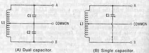
Fig. 11. Symmetrical-tuned circuits. (A) Dual capacitor. (B) Single capacitor.

11. DC-TUNED CIRCUITS

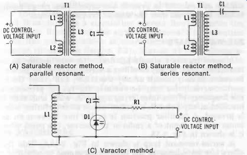
Fig. 12. Tuned, dc controlled circuits. (A) Saturable reactor method, parallel resonant. (B) Saturable reactor method, series resonant. (C) Varactor method.

Certain LC circuits can be tuned by means of an adjustable dc voltage. This is convenient in remote tuning, remote control of apparatus, automatic frequency control (afc), and various automation processes aid telemetering. Fig. 12 shows two methods.

A saturable reactor (T,) is employed in Fig. 12A and B.

In this transformer-like device, dc flowing through the primary winding (L1 and L2 in series) changes the permeability of the core and thereby changes the inductance of the secondary winding (L3). The resonant circuit is comprised of secondary coil L3 and capacitor C1. The secondary and capacitor are connected for parallel resonance in Fig. 12A, and for series resonance in Fig. 12B. Primary coils L1 and I, are connected in series bucking, so that no ac from the secondary is fed back to the dc control-voltage source. The sensitivity of the circuit is such that a small direct current flowing through the primary winding can control a large alternating current in the L3C1 tank. Special core materials afford operation at high frequencies.

A varactor (voltage-variable capacitor), D1, is employed in Fig. 12C. This is a specially processed silicon diode which is operated in the reverse-biased mode (anode negative, cathode positive). In this circuit, the resonant frequency is determined by the inductance of coil L1 and the dc-controlled capacitance of the varactor. Capacitor C1 is a blocking capacitor which prevents the coil from short-circuiting the dc control voltage; its capacitance is chosen much higher than that of the varactor (usually 1000 x) for lowest reactance, so that the varactor-rather than capacitor C1--tunes the circuit.

Isolating resistance R1 is very high (usually 1 to 10 meg ohms) ; and since the varactor is essentially voltage operated, there is virtually no current through this resistor and accordingly no voltage drop across it. The varactor and dc control voltage are selected to provide the capacitance range needed to tune the circuit over the desired frequency range.

12. WAVE TRAPS

A wave trap is a simple LC device for eliminating an interfering signal. It may be either a series-resonant or parallel-resonant circuit, though usually the latter, and either the capacitor or inductor may be variable for tuning precisely to the frequency of the interfering signal. A wave trap may be installed at any point in a system where an interfering signal is present. A familiar position is in the line between an antenna and the input of a radio or tv receiver, the point where it is shown in Fig. 13.

A series-resonant trap is shown in Fig. 13A. This trap offers low impedance to the interfering signal to which it is tuned, and the signal accordingly is shunted around the receiver to ground. Signals of other frequencies see the trap as a higher impedance, and pass by it to the receiver, with little loss. A parallel-resonant trap is shown in Fig. 13B.

This trap offers high impedance to the interfering signal which it captures as a circulating current flowing inside the L1C1 tank. Removal of the signal corresponds to reduction of the line current, which is characteristic of the parallel-resonant circuit (see Section 2). Signals at other frequencies see the trap as a lower impedance, and pass through to the receiver with little loss. In either type of trap, the circuit Q must be as high as practicable, to minimize attenuation of desired signals. Another familiar position for one or more wave-traps is the output circuit of a transmitter, where the trap removes undesired harmonics of the radiated signal.

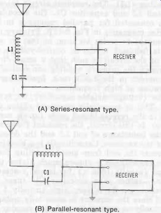
Fig. 13. Wave traps. (A) Series-resonant type. (B) Parallel-resonant type.

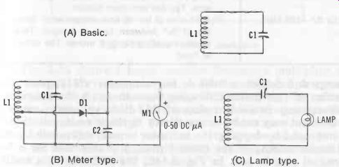
Fig. 14. Wave-meters. (A) Basic. (B) Meter type. (C) Lamp type.

-----------

Table 2-1. Wavemeter Coil Data

Variable Capacitor C, = 140 pF (A) 1.1-3.8 MHz 72 turns No. 32 enameled wire close-wound on 1"-diameter plug-in form. Tap 18th turn from bottom.

(B) 3.7-12.5 MHz 21 turns No. 22 enameled wire close-wound on 1"-diameter plug-in form. Tap 7th turn from bottom. (C) 12-39 MHz 6 turns No. 22 enameled wire on 1"-diameter plug-in form. Space to winding length of 3/8 inch. Tap 3rd turn from bottom.

(D) 37-150 MHz Hairpin loop of No. 16 bare copper wire. Spacing of 1/2" between legs of hairpin. Total length including bend: 2 inches Tap center of bend.

-------------

13. WAVEMETERS

Another familiar application of the simple LC tuned circuit is the absorption wavemeter, so called because its operation depends upon its absorption of a small amount of rf energy from the circuit to which it is inductively coupled. This instrument is also called an absorption frequency meter.

Fig. 14 shows three common versions of this instrument.

Basically, it, like the wave trap, is a single-tuned circuit consisting of a fixed-inductance coil (L1) and variable capacitor (C1). The coil is loosely coupled to the tank of the oscillator or amplifier under test, by holding it near the latter, and the wavemeter is tuned to resonance at the unknown frequency (fr) by adjusting the capacitor. The unknown frequency then is read from the calibrated dial of the capacitor. The frequency range (band) is changed by plugging in a different coil.

Resonance can be indicated in several ways. When the circuit in Fig. 14A is used, the unknown-signal source must have a current meter in its output stage (a plate milliammeter in a tube-type source, a collector milliammeter in a transistor-type source), and the deflection of this meter will rise sharply as the wavemeter is tuned, the peak point of this rise indicating resonance. In the two other arrangements--Figs. 14B and C-the wavemeter has a self-contained indicator. In Fig. 14B, a germanium diode (D1) rectifies the picked-up rf energy and deflects a 0-50-dc microammeter (M1), peak deflection of this meter indicating resonance. (A thermo-galvanometer may be used in place of this diode and meter combi nation, but may not be so sensitive.) In this circuit, selectivity is improved by tapping the indicator circuit down coil L1 to minimize loading of the tuned circuit. But this calls for a 3-terminal plug-in coil. In Fig. 14C, the indicator is a small pilot lamp, such as the 2-V, 60-mA Type 48. This arrangement can be used only when the signal source-such as a radio transmitter or industrial oscillator-supplies enough power to light the lamp. In this arrangement, peak brilliance of the lamp indicates resonance.

Table 2-1 gives coil-winding data for a wavemeter employing a 140-pF tuning capacitor. The four inductors cover the frequency spectrum of 1.1 to 150 MHz in four bands. Other inductance and capacitance combinations may be worked out for other frequencies (see Equations 1, 2, and 3).

14. VARACTOR FREQUENCY MULTIPLIER

The varactor was introduced in Section 11 in its role as a dc-variable capacitor for resonant-circuit tuning. The most important large-signal application of the varactor in company with LC tuned circuits is harmonic generation. The latter property arises as a result of the pronounced distortion occurring when the varactor is operated over its entire range of nonlinear response. This property is utilized in modern high-efficiency passive frequency doublers, triplers, quadruplers, and higher-order multipliers in transmitters and other radio-frequency equipment.

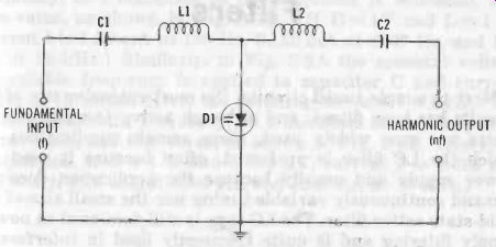
Fig. 15. Basic varactor multiplier.

Fig. 15 shows a basic varactor frequency multiplier circuit. Input (driving) current at the fundamental frequency (f) flows through the left loop (C1L1D1) of the circuit.

Series-resonant circuit L1C1 is tuned to this frequency. Flow of this current through the varactor generates a number of harmonics. The desired harmonic (nf) is selected by the second series-resonant circuit (L2C2) and is delivered to the HARMONIC OUTPUT terminals.

Every varactor multiplier circuit is some adaptation of the simple arrangement shown in Fig. 15; some, for instance, employ parallel-resonant circuits. The varactor multiplier is not only efficient (PO/P, approaches 100% for doublers, where P is output power, and P, is input power, both radio-frequency), but it also requires no local power supply. The only power required for its operation is supplied by the input signal itself.