There are two aspects to oscilloscope performance: the design parameters of the instrument, and its conformance to those parameters at the time you are making measurements. Making the instrument conform to its de sign parameters simply means calibration — including making sure the probe is properly compensated as you’ve done many times already. But even with proper calibration, there will be some effect of the designed performance on your measurements.
AMAZON multi-meters discounts AMAZON oscilloscope discounts
Square Wave Response and High Frequency Response
In the design of amplifiers like those in a scope’s vertical channels, there is always some compromise between the circuit’s high frequency response and its handling of signals with square transitions. Extending the frequency response can be accomplished with high frequency compensation, but too much compensation results in overshoot on a step. Too little extends the measured rise time. The best rise times without over shoot are achieved when the high frequency response is critically damped; the frequency response then falls off smoothly Figure 32 illustrates the effects of high frequency compensation.
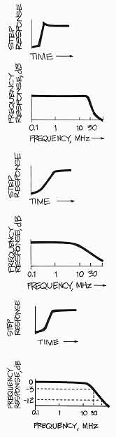
Figure 32. HIGH FREQUENCY COMPENSATION in a scope’s vertical amplifier has an
effect: on the rise time of square waves measured by the scope. If too much
high frequency compensation is present, the rise times will show overshoot and possible ringing, as in the top drawing. Too little, as shown in the second
drawing, tends to rolloff the edges of the square wave. A critically damped
frequency response is best as in the third drawing.
Instrument Rise Time and Measured Rise Times
The rise time of an oscilloscope is a very important specification because the measuring instrument’s rise time affects the ac curacy of your measured rise times as expressed by this approximation:
Tr(measurement) =
![]()
In practical terms this means that the accuracy of a measured signal will be predictable and will be dependent on how much faster your scope is than the rise time you’re measuring. If the measuring scope is five times faster than the observed signal, the measurement error can be as low as 2%. For measurement accuracies of 1 %, it takes a scope 7 times faster, as you can see on the chart in Figure 33.
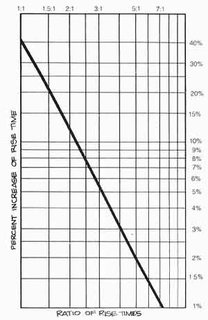
Figure 33. MEASURED RISE TIME ERRORS depend on the ratio of the measuring
system’s rise time to the rise time of the signal being measured. As you
can see from the chart, when the scope is five times faster the error is a
2% increase in the measured rise time. If the rise times are equal, the error
is a 41% increase.
Bandwidth and Rise Time
The vertical channels of an oscilloscope are designed for a broad band pass, generally from some low frequency (DC) to a much higher frequency. This is the oscilloscope’s bandwidth, specified by listing the frequency at which a sinusoidal input signal has been attenuated to 0.707 of the middle frequencies; this is called the -3 dB point. For older instruments, specifications cited both a low and high -3 dB point. Modern instruments, however, have a relatively flat frequency response down to 0 Hz (DC), so only the upper number is quoted as the bandwidth.
A bandwidth specification gives you an idea of instrument’s ability to handle high frequency signals within a specified attenuation. But bandwidth specifications are derived from the instrument’s ability to display sine waves. A 35 MHz scope will show a 35 MHz sine wave with only -3 dB attenuation, but the effects on a square wave at or near the scope’s upper bandwidth limit will be much more severe because high frequency information in the square wave will not be accurately reproduced by the scope. See Figure 34 for an example.
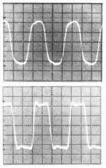
Figure 34. BANDWIDTH SPECIFICATIONS are based on the scope’s ability to
repro duce sine waves. The upper bandwidth is the frequency at which a sine
wave is reduced to 0.707 of the amplitude shown at middle frequencies. Though
this specification tells you how well the instrument reproduces sine waves,
not every signal you examine is sinusoidal. Square waves, for example. have
a great deal of high frequency information in their rising and falling edges
that will be lost as you approach the bandwidth limits of the instrument.
To illustrate, the two CAT photos show a 15 MHz square wave reproduced
by 35 MHz (top) and 60 MHz (bottom) oscilloscopes.
The frequency response of most scopes is designed so that there is a constant that allows you to relate the bandwidth and rise time of the instrument. This constant is 0.35 and the rise time and bandwidth are related by this approximation:
Tr = 0.35/(BW)
A simple way to apply the formula is:
Tr(nanoseconds) = 350 / BW(megahertz)
For the Tektronix 2200 Series instruments with a bandwidth of 60 MHz, the rise time is 5.8 nanoseconds.
CONCLUSION
This concludes your introduction to oscilloscopes and the measurements you can make with scopes. You’ve done well to progress this far, but this primer can only introduce the concepts and measurement techniques. With practice and experience, you’ll find yourself making faster and more accurate measurements. Then you too will find that using an oscilloscope is second nature to you.