Using an Oscilloscope: Part II. Section 9. MEASUREMENT TECHNIQUES

Rather than attempt to describe how to make every possible measurement, this section de scribes common measurement techniques you can use in many applications.

The Foundations: Amplitude and Time Measurements

The two most basic measurements you can make are amplitude and time; almost every other measurement you’ll make is based on one of these two fundamental techniques.

Since the oscilloscope is a voltage-measuring device, volt age is shown as amplitude on your scope screen. Of course, voltage, current, resistance, and power are related:

Current = voltage / resistance

Resistance = voltage / current

Power = current x voltage

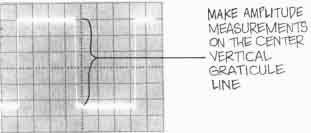
Amplitude measurements are best made with a signal that covers most of the screen vertically. Use Exercise 6 to practice making amplitude measurements.

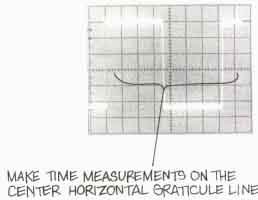
Time measurements are also more accurate when the signal covers a large area of the screen. Continue with the set-up you had for the amplitude measurement, but now use Exercise 7 (below) to make a period measurement.

Exercise 6. AMPLITUDE MEASUREMENTS

1. Connect your probe to the channel 1 BNC connector and to the probe adjustment jack. Attach the probe ground strap to the collar of the channel 2 BNC. Make sure your probe is compensated and that all the variable controls are set in their detent positions.

2. The trigger MODE switch should be set to NORM for nor mal triggering, the HORIZONTAL MODE should be NO DLY (A on the 2215A). Make sure the channel 1 coupling switch is set to AC and that the trigger SOURCE switch is on internal and the INT switch on CH1. Set the VERTICAL MODE switch to CH 1 as well.

3. Use the trigger LEVEL control to obtain a stable trace and move the volts/division switch until the probe adjust square wave is about five divisions high. Now turn the seconds / division switch until two cycles of the waveform are on your screen. (The settings should be 0.1 V on the VOLTS/DIV and0.2 ms on the SEC/DIV switches.)

4. Now use the CH 1 vertical POSITION control to move the square wave so that its top is on the second horizontal graticule line from the top edge of the screen. Use the horizontal position control to move the signal so that the bottom of one cycle intersects the center vertical graticule line.

5. Now you can count major and minor divisions down the center vertical graticule line and multi ply by the VOLTS/DIV setting to make the measurement. For example, 5.0 divisions times 0.1 volts equals 0.5 volts. (If the voltage of the probe adjustment square wave in your scope is different from this example, that’s because this signal is not a critical part of your scope and tight tolerances and exact calibration are not required.).

Exercise 7. TIME MEASUREMENTS

Time measurements are best made with the center horizontal graticule line. Use the instrument settings from Exercise 6 and center the square wave vertically with the vertical POSITION control. Then line up one rising edge of the square wave with the graticule line that’s second from the left-hand side of the screen with the HORIZONTAL position control, Make sure the next rising edge intersects the center horizontal graticule. Count major and minor divisions across the center horizontal graticule line from left to right as shown in the photo above. Multiply by the SEC/DIV setting; for example, 5.7 divisions times 0.2 milliseconds equals 1.14 milliseconds. (if the period of the probe adjustment square wave in your scope is different from this example, remember that this signal is not a critical part of the calibration of your scope.)

Frequency and Other Derived Measurements

The voltage and time measurements you just made are two examples of direct measurements. Once you’ve made a direct measurement, there are de rived measurements you can calculate. Frequency is one example; it’s derived from period measurements. While period is the length of time required to complete one cycle of a periodic waveform, frequency is the number of cycles that take place in a second. The measurement unit is a hertz (1 cycle/second) and it’s the reciprocal of the period. So a period of 0.00114 second (or 1.14 milliseconds) means a frequency of 877 Hz.

More examples of derived measurements are the alternating current measurements illustrated by Figure 24.

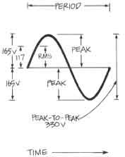
Figure 24. DERIVED MEASUREMENTS are the result of calculations made after direct measurements. For example, alternating current measurements require an amplitude measurement first. The easiest place to start is with a peak-to- peak amplitude measurement of the voltage in this case, 330 volts because peak-to-peak measurements ignore positive and negative signs. The peak voltage is one-half that (when there is no DC offset), and is also called a maximum value; it’s 165 V in this case. The average value is the total area under the voltage curves divided by the period in radians; in the case of a sine wave, the average value is 0 because the positive and negative values are equal. The RMS (root mean square) voltage for this sine wave which represents the line volt age in the United States is equal to the maximum value divided by the square root of 2: 165 / 1.414 = 117volts. You get from peak-to-peak to RMS volt age with: peak-to-peak / 2x the square root of 2.

Pulse Measurements

Pulse measurements are important when you work with digital equipment and data communications devices. Some of the signal parameters of a pulse were shown in Figure 20, but that was an illustration of an ideal pulse, not one that exists in the real world. The most important parameters of a real pulse are shown in Figure 25.

Use Exercise 8 to make derived measurements with the probe adjustment square wave.

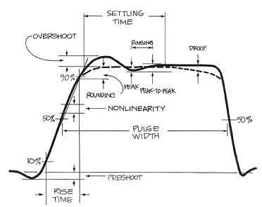
Figure 25. REAL PULSE MEASUREMENTS include a few more parameters than those for an ideal pulse. In the diagram above, several are shown. Pre-shooting is a change of amplitude in the opposite direction that precedes the pulse. Overshooting and rounding are changes that occur after the initial transition. Ringing is a set of amplitude changes usually a damped sinusoid that follows overshooting. All are expressed as percentages of amplitude. Settling time expresses how long it fakes the pulse to reach it maximum amplitude. Droop is a decrease in the maximum amplitude with time. And nonlinearity is any variation from a straight line drawn through the 10 and 90% points of a transition.

Exercise 8. DERIVED MEASUREMENTS

With the period measurement you just made in Exercise 7, calculate the frequency of the probe adjustment square wave. For example, if the period is 1 millisecond, then the frequency is the reciprocal, 1/0.001 or 1000 Hz. Other derived measurements you can make are duty cycle, duty factor, and repetition rate. Duty cycle is the ratio of pulse width to signal period ex pressed as a percentage: 0.5 ms / 1 ms, or 50%. But you knew that because for square waves, it’s always 50%. Duty factor is 0.5. And the repetition rate (describing how often a pulse train occurs) is 1000/second in this case because repetition rate and frequency are equal for square waves. Your probe adjustment signal might differ slightly from this example; calculate the derived measurements for it. You can also calculate the peak, peak-to-peak, and average values of the probe adjustment square wave in your scope. Don’t forget that you need both the alternating and direct components of the signal to make these measurements, so be sure to use direct coupling (DC) on the vertical channel you’re using.

Use the directions in Exercise 9 to make a pulse measurement on the probe adjustment square wave.

Exercise 9. PULSE WIDTH MEASUREMENTS

To measure the pulse width of the probe adjustment square wave quickly and easily, set your scope to trigger on and display channel 1. Your probe should still be connected to the channel 1 BNC connector and the probe adjustment jack from the previous exercises. Use 0.1 ms/division and the no delay horizontal mode (A sweep if you’re using a 2215A). Use P-P AUTO triggering on the positive slope and adjust the trigger LEVEL control to get as much of the leading edge as possible on your screen. Switch the coupling on channel 1 to ground and center the baseline on the center horizontal graticule. Now use AC coupling because that will center the signal on the screen and you make pulse width measurements at the 50% point of the waveform. Use your horizontal POSITION control to line up the 50% point with the first major graticule from the left side of the screen. Now you can count divisions and subdivisions across the center horizontal and multi ply by the SEC/DIV switch set ting to find the pulse width.

Phase Measurements

You know that a waveform has phase, the amount of time that has passed since the cycle began, measured in degrees. There is also a phase relation ship between two or more waveforms: the phase shift (if any). There are two ways to measure the phase shift between two waveforms. One is by putting one waveform on each channel of a dual-channel scope and viewing them directly in the chop or alternate vertical mode; trigger on either channel. Adjust the trigger LEVEL control for a stable display and mea sure the period of the wave forms. Then increase the sweep speed so that you have a display something like the second drawing back in Figure 22.Then measure the horizontal distance between the same points on the two waveforms. The phase shift is the difference in time divided by the period and multiplied by 360 to give you degrees.

Displaying the two waveforms and measuring when one starts with respect to another is possible with any dual trace scope, but that isn’t the only way to make a phase measurement. Look at the front panel and you’ll see that the vertical channel BNC connectors are labeled X and Y. The last position on the SEC/DIV switch is XY, and when you use it, the scope’s time base is bypassed. The channel 1 input signal is still the vertical axis of the scope’s display, but now the signal on channel 2 be comes the horizontal axis. In the X-Y mode, you can input one sinusoidal on each channel and your screen will display a Lissajous pattern. (They are named for Jules Antoine Lissajous, a French physicist; say “LEE-za shu”). The shape of the pattern will indicate the phase difference between the two signals. Some examples of Lissajous patterns are shown in Figure 26.

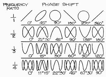
Figure 26. FREQUENCY MEASUREMENTS WITH LISSAJOUS PATTERNS require a known sine wave on one channel. If there is no phase shift, the ratio between the known and unknown signals will correspond to the ratio of horizontal and vertical lobes of the pattern. When the frequencies are the same, only the shifts in phase will affect the pattern. In the drawings above, both phase and frequency differences are shown.

Note that general purpose oscilloscope Lissajous pattern phase measurements are usually limited by the frequency response of the horizontal amplifier (typically designed with far less bandwidth than vertical channels). Specialized X-Y scopes or monitors will have al most identical vertical and horizontal systems.

X-Y Measurements Finding the phase shift of two sinusoidal signals with a Lissajous pattern is one example of an X-Y measurement. The X-Y capability can be used for other measurements as well. The Lissajous patterns can also be used to determine the frequency of an unknown signal when you have a known signal on the other channel. This is a very accurate frequency measurement as long as your known signal is accurate and both signals are sine waves. The pat terns you can see are illustrated in Figure 26, where the effects of both frequency and phase differences are shown. Component checking in ser vice or production situations is another X-Y application; it re quires only a simple transistor checker like that shown in Figure 27.

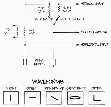
Figure 27. X-Y COMPONENT CHECKING requires the transistor checker shown above. With it connected to your scope and the scope in the X-Y mode, patterns like those illustrated indicate the component’s condition. The waveforms shown are found when the components are not in a circuit; in-circuit component patterns will differ because of resistors and capacitors associated with the component.

There are many other applications for X-Y measurements in television servicing, in engine analysis, and in 2-way radio servicing, for examples. In fact, any time you have physical phenomena that are interdependent and not time-dependent, X-Y measurements are the answer. Aerodynamic lift and drag, motor speed and torque, or pressure and volume of liquids and gasses are more examples. With the proper transducer, you can use your scope to make any of these measurements.

Differential Measurements

The ADD vertical mode and the channel 2 INVERT button of your 2200 Series scope let you make differential measurements. Often differential measurements let you eliminate undesirable components from a signal that you’re trying to measure. If you have a signal that’s very similar to the unnecessary noise, the set up is simple. Put the signal with the spurious information on channel 1. Connect the signal that's like unwanted components to channel 2. Set both input coupling switches to DC (use AC if the DC components of the signal are too large), and select the alternate vertical mode by moving the VERTICAL MODE switches to BOTH and ALT.

Now set your volts/division switches so that the two signals are about equal in amplitude. Then you can move the right- hand VERTICAL MODE switch to ADD and press the INVERT button so that the common mode signals have opposite polarities.

If you use the channel 2 VOLTS/DIV switch and CAL control for maximum cancellation of the common signal, the signal that remains on-screen will only contain the desired part of the channel 1 input signal. The two common mode signals have cancelled out leaving only the difference between the two.

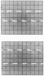
Figure 28. DIFFERENTIAL MEASUREMENTS allow you to remove unwanted information from a signal anytime you have another signal that closely resembles the unwanted components. For example, the first photo shows a 1 kHz square contaminated by a 60Hz sine wave. Once the common-mode component (the sine wave) is input to channel 2 and that channel is inverted, the signals can be added with the ADD vertical mode. The result is shown in the second photo.

Using the Z Axis

Remember from Part I that the CRT in your scope has three axes of information: X is the horizontal component of the graph, Y is the vertical, and Z is the brightness or darkness of the electron beam. The 2200 Series scopes all have an external Z-axis input BNC connector on the back of the instrument. This input lets you change the brightness (modulate the intensity) of the signal on the screen with an external signal. The Z-axis input will accept a signal of up to 30 V through a usable frequency range of DC to 5 MHz. Positive voltages decrease the brightness and negative volt ages increase it; 5 volts will cause a noticeable change. The Z-axis input is an advantage to users that have their instruments set up for a long series of tests. One example is the testing of high fidelity equipment illustrated by Figure 29.

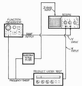
Figure 29. USING THE Z-AXIS can provide additional information on the scope screen. In the set-up drawn above, a function generator sweeps through the frequencies of interest during the product testing—20 to 20,000 Hz, in this case. Then an adjustable notch filter is used to generate a marker, at 15 kHz, for instance, and this signal is applied to the Z-axis input to brighten the trace. This allows the tester to evaluate the product’s performance with a glance.

Using TV Triggering

The composite video waveform consists of two fields, each of which contains 262 lines. Many scopes offer television triggering to simplify looking at video signals. Usually, however, the scope will only trigger on fields at some sweep speeds and lines at others. The 2200 Series scopes allow you to trigger on either lines or fields at any sweep speed.

To look at tv fields with a 2200 Series scope, use the TV FIELD mode. This mode allows the scope to trigger at the field rate of the composite video signal on either field one or field two. Since the trigger system can't recognize the difference between field one and field two, it will trigger alternately on the two fields and the display will be confusing if you look at one line at a time.

To prevent this, you add more holdoff time, and there are two ways to do that. You can use the variable holdoff control, or you can simply switch the vertical operating mode to display both channels. That makes the total holdoff time for one channel greater than one field period. Then just position the unused vertical channel off-screen to avoid confusion.

It is also important to select the trigger slope that corresponds to the edge of the waveform where the sync pulses are located. Picking a negative slope for pulses at the bottom of the waveform allows you to see as many sync pulses as possible.

When you want to observe the TV line portion of the composite video signal, use the TV-LINE trigger mode and trigger on the horizontal synchronization pulses for a stable display. It is usually best to select the blanking level of the sync waveform so that the vertical field rate will not cause double triggering.

Delayed Sweep Measurements

Delayed sweep is a technique that adds a precise amount of time between the trigger point and the beginning of a scope sweep. Often delayed sweep is used as a convenient way to make a measurement (the rise time measurement in Exercise 10 is a good example). To make a rise time measurement without delayed sweep, you must trigger on the edge occurring be fore the desired transition. With delayed sweep, you may choose to trigger anywhere along the displayed waveform and use the delay time control to start the sweep exactly where you want.

Sometimes, however, delayed sweep is the only way to make a measurement. Suppose that the part of the waveform you want to measure is so far from the only available trigger point that it will not show on the screen. The problem can be solved with delayed sweep: trigger where you have to, and delay out to where you want the sweep to start.

But the delayed sweep feature you’ll probably use the most often is the intensified sweep; it lets you use the delayed sweep as a positionable magnifier. You trigger normally and then use the scope’s intensified horizontal mode. Now the signal on the screen will show a brighter zone after the delay time. Run the delay time (and the intensified zone) out to the part of the signal that interests you. Then switch to the delayed mode and increase the sweep speed to magnify the selected waveform portion so that you can examine it in detail.

Since the 2200 Series has two types of delayed sweep, read the paragraphs and use the delayed sweep measurement exercise below that applies to your scope: “Single Time Base Scopes” and Exercise 10 for delayed sweep measurements with single time base scopes like the Tektronix 2213A; or “Dual Time Base Scopes” and Exercise 11 for delayed sweep on dual time base scopes like the 2215A.

Single Time Base Scopes

Very few single time base scopes offer delayed sweep measurements. Those that do may have measurement capabilities similar to those of the Tektronix 2213A which has three possible horizontal operating modes annotated on the front panel as NO DLY, INTENS, and DLY’D.

When you set the HORIZONTAL MODE switch to NO DLY (no delay), only the normal sweep functions.

When you choose INTENS (intensified sweep), your scope will display the normal sweep and the trace will also be intensified after a delay time. The amount of delay is determined by both the DELAY TIME switch (you can use 1.0 s, 20 s, or 0.4 ms) and the DELAY TIME MULTIPLIER control. The multiplier lets you pick from 1 to 50 times the switch setting.

The third position, DLY’D (delayed), makes the sweep start after the delay time you’ve chosen. After selecting this position you can move the SEC/DIV to a faster sweep speed and examine the waveform in greater detail.

This list of horizontal modes should begin to give ideas of how useful these delayed sweep features are. Start by making the rise time measurement described below. (Note that when making rise time measurements, you must take the rise time of the measuring instrument into account. Be sure to read Section 10.)

Dual Time Base Scopes

Delayed sweep is normally found on dual time base scopes like the 2215A with two totally separate horizontal sweep generators. In dual time base instruments, one sweep is triggered in the normal fashion and the start of the second sweep is delayed. To keep these two sweeps distinct when de scribing them, the delaying sweep is called the A sweep; the delayed sweep is called the B sweep. The length of time between the start of the A sweep and the start of the B sweep is called the delay time.

Dual time base scopes offer you all the measurement capabilities of single time base instruments, plus:

• convenient comparisons of signals at two different sweep speeds

• jitter-free triggering of delayed sweeps

• and timing measurement ac curacy of 1.0%.

Most of this increase in measurement performance is avail able because you can separately control the two sweep speeds and use them in three horizontal operating modes. These modes—in a 2215A— are A sweep only, B sweep only, or A intensified by B as well as B delayed. The HORIZONTAL MODE switch controls the operating mode and two SEC/DIV switches — concentrically mounted on a 2215A—control the sweep speeds. See Figure 30.

When you use the ALT (for al ternate horizontal mode) position the HORIZONTAL MODE switch, the scope will display the A sweep intensified by the B sweep and the B sweep delayed. As you set faster sweeps with the B SEC/DIV switch, you’ll see the intensified zone on the A trace get smaller and the B sweep expanded by the new speed setting. As you move the B DELAY TIME POSITION dial and change where the B sweep starts, you’ll see the intensified zone move across the A trace and see the B waveform change.

This sounds more complicated in words than it's in practice. As you use the scope in Exercise 11, you’ll find that the procedure is very easy. You will always see exactly where the B sweep starts. And you can use the size of the intensified zone to judge which B sweep speed you need to make the measurement you want.

Exercise 10. 2213 DELAYED SWEEP MEASUREMENTS

1. Connect your probe to the channel 1 BNC connector and the probe adjustment jack, hook the ground strap onto the collar of the channel 2 BNC, and make sure the probe is compensated. 2. Use these control settings:

CH1 VOLTS/DIV on 0.2 using the 10X probe VOLTS/DIV read out, CH1 input coupling on AC, VERTICAL MODE is CH1; TRIGGER MODE is P-P AUTO; TRIGGER SLOPE is negative (—); trigger SOURCE is INT (for internal) and INT trigger switch is either CH1 or VERT MODE; HORIZONTAL MODE is NO DLY; SEC/DIV is 0.5 ms. Check all the variable controls to make sure they’re in their calibrated detent positions.

3. Set the input coupling to GND and center the trace. Switch back to AC and set the trigger LEVEL control for a stable display. The waveform should look like the first photo above.

4. Because a rise time measurement is best made at faster sweep speeds, turn the SEC/DIV control to 2 uS (micro-seconds). Use the trigger LEVEL control to try to get all of the positive transition on the screen. You can’t; you lose your trigger when you get off the slope of the signal.

5. Turn back to 0.5 ms/div and switch to the intensified display with the HORIZONTAL MODE switch. Switch the DELAY TIME to 0.4 ms and use the DELAY TIME MULTIPLIER to move the intensified zone on the waveform to a point before the first complete positive-going transition of the square wave. The intensified zone now shows you where the delayed sweep will start, like the second photo.

6. Switch the horizontal mode to DLY’D and the SEC/DIV switch to 5 uS. Now you can use the horizontal POSITION and DELAY TIME MULTIPLIER controls to get a single transition on the screen.

8. Use the horizontal POSITION control to move the waveform until it crosses a vertical graticule line at the 10% marking. Adjust the FOCUS control for a sharp waveform and make your rise time measurement from that vertical line to where the step crosses the 90% line. Now you can make a rise time measurement on a waveform like that in the third photograph. For example, for 1 major division and 4 minor divisions: 1.8 times the SEC/DIV setting of 5 uS is 9 uS.

7. Change to 0.1 V/div and line up the signal with the 0 and 100% dotted lines of the graticule. (If you have a signal that doesn’t fit between the 0 and 100% lines of the graticule, you have to count major and minor divisions and estimate the rise time while ignoring the first and last 10% of the transition.)

Measurements at Two Sweep Speeds

Looking at a signal with two different sweep speeds makes complicated timing measurements easy. The A sweep gives you a large slice of time on the signal to examine. The intensified zone will show you where the B sweep is positioned. And the faster B sweep speeds magnify the smaller portions of the signal in great detail. You’ll find this capability useful in many measurement applications; see Figure 31 for two illustrations.

Because you can use the scope to show A and B sweeps from both channel 1 and channel 2, you can display four traces. To prevent overlapping traces, most dual time base scopes offer an additional position control. On the 2215A it’s labeled ALT SWP SEP for alternate sweep separation. With it and the two vertical channel POSITION controls, you can place all four traces on-screen without confusion.

Separate B Trigger

Jitter can prevent an accurate measurement anytime you want to look at a signal that isn’t perfectly periodic. But with two time bases and delayed sweep, you can solve the problem with the separate trigger available for the B sweep. You trigger the A sweep normally and move the intensified zone out to the portion of the waveform you want to measure. Then you set the scope up for a triggered B sweep, rather than letting the B sweep simply run after the delay time.

On a 2215A, the B TRIGGER LEVEL control does double duty. In its full clockwise position, it selects the run-after delay mode. At any other position, it functions as a trigger level control for the B trigger. The B TRIGGER SLOPE control lets you pick positive or negative transitions for the B trigger.

With these two controls you can trigger a stable B sweep even when the A sweep has jitter.

Increased Timing Measurement

Accuracy Besides examining signals at two different sweep speeds and seeing a jitter-free B sweep, you get increased timing measurement accuracy with a dual time base scope.

Note that the B DELAY TIME POSITION dial is a measuring indicator as well as a positioning device. The numbers in the window at the top of the dial are calibrated to the major divisions of the scope screen. The numbers around the circumference divide the major division into hundreds.

To make timing measurements accurate to 1.0% with the B DELAY TIME POSITION dial:

• use the B runs-after-delay mode.

• place the intensified zone (or use the B sweep waveform) where the timing measurement begins, and note the B DELAY TIME POSITION dial setting

• dial back to where the measurement ends and note the reading there

• subtract the first reading from the second and multiply by the A sweep SEC/DIV setting.

You’ll find an example of this accurate—and easy—timing measurement in Exercise 11.

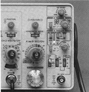
Figure 30. THE DELAYED SWEEP CONTROLS of the dual time base 2215A are shown on the photograph above. They include: HORIZONTAL MODE (under the horizontal POSI TION control); B TRIGGER SLOPE and LEVEL; ALT SWP SEP (alternate sweep separation, between the two vertical POSITION controls—not shown), and a concentric A and B SEC/DIV control. The B DELAY TIME POSITION dial is at the bottom of the column of horizontal system controls.

Figure 31. ALTERNATE DELAYED SWEEP MEASUREMENTS are fast and accurate One use examining timing in a digital circuit, is demonstrated in the first photograph Suppose you need to check the width of one pulse in a pulse train like the one shown To make sure which pulse you are measuring you want to look at a large portion of a signal But to measure the one pulse accurately, you need a faster sweep speed Looking at both the big picture and a small enlarged portion of the signal is easy with alternate delayed sweep Another example is shown in the second photo. Here one field of a composite video signal is shown in the first waveform. The intensified portion of that field is the lines magnified by the faster B sweep With a dual time base scope, you can walk through the field with the B DELAY TIME POSITION dial and look at each line individually

Exercise 11. 2215A DELAYED SWEEP MEASUREMENTS

Rise Time Measurement

1. Connect your probe to the channel 1 BNC connector and the probe adjustment jack, hook the ground strap onto the collar of the channel2 BNC, and make sure the probe is compensated. 2. Use these control settings:

CH 1 VOLTS/DIV on 0.2 (re member to use the 10X probe readout); CH 1 input coupling on AC; VERTICAL MODE is CH 1; A TRIGGER MODE is NORM; A TRIGGER SLOPE is negative (—); A SOURCE is INT and the A&B INT trigger switch is either CH 1 or VERT MODE; HORIZONTAL MODE is A; A and B SEC/DIV is 0.2 ms. Check the variable controls to make sure they’re in their calibrated detent positions.

3. Set the A TRIGGER LEVEL control for a stable display and position the waveform in the top half of the screen. Switch to the ALT (for alternate A and B sweeps) display with the HORIZONTAL MODE switch. Use the channel 1 POSITION and ALT SWP SEP (alternate sweep separation) controls to position the two sweeps so that they don’t overlap.

4. Use the B DELAY TIME POSI TION dial to move the beginning of the intensified zone a point before the first complete positive transition. Your screen should look like the first photo above.

5. Pull out on the SEC/DIV knob and rotate it clockwise to change the B sweep speed to 2 uS/division. This will make the intensified zone smaller; move it to the first rising edge of the waveform as in the second photograph.

6. Switch the horizontal mode to B, the channel 1 vertical sensitivity to 0.1 volts/division, and the sweep speed to 1 us/division. Use the horizontal and vertical POSITION controls and the B DELAY TIME POSITION control to line up the waveform with the 0 and 100% dotted lines of the graticule. (If you have a signal that doesn’t fit between the 0 and 100% lines of the graticule, you have to count major and minor divisions and estimate the rise time while ignoring the first and last 10%.)

7. Position the waveform so that it crosses a vertical graticule line at the 10% marking. Adjust the FOCUS and the B INTENSITY control for a sharp, bright wave form and count major and minor divisions across the screen to where the step crosses the 90% line. If there are 4 major and 8 minor divisions, 4 and 8/10 times the SEC/DIV setting of 1 uS is 4.8 uS. The third photo shows how the screen should look now. (Note: Any jitter you see in the B sweep is from the probe adjustment circuit, not the time base.)

8. One last word on rise time measurements: the accuracy of the measurement you make depends on both the signal you’re examining and the performance of your scope. In Section 10, you’ll find a description of how the scope’s own rise time affects your measurement results.

Pulse Width Measurement

1. Use these control settings:

CH1 VOLTS/DIV on 0.1; CH1 input coupling on AC; VERTICAL MODE is CH 1; A TRIGGER MODE is NORM; A TRIGGER SLOPE is negative (—); A TRIGGER SOURCE is INT (for internal) and INT trigger switch is either CH 1 or VERT MODE; HORIZONTAL MODE is A; A SEC/DIV is 0.2 ms while B SEC/DIV is 0.05 uS. Check the variable controls.

2. Center the first complete pulse of the waveform horizon tally. Switch to the ALT display with the HORIZONTAL MODE switch and move the B waveform to the bottom of the screen with the ALT SWP SEP control.

3. Center A sweep waveform vertically. Turn down the intensity so that it’s easier to see the small intensified zone.

4. Move the intensified zone to the 50% point of the rising edge of the waveform with the DELAY TIME POSITION control as in the first photo above. Note the delay time reading (the number in the window first, for example: 3.1). Move the intensified zone to the 50%point of the trailing edge as in the second photo and note the reading.

5. The time measurement, a pulse width in this case, is equal to the second dial reading minus the first times the A sweep speed: 5.77 — 3.13 x 0.2 ms = 0.528 ms. In other words, the B DELAY TIME POSITION dial indicates screen divisions for you, 1 complete turn for every major division.