AMAZON multi-meters discounts AMAZON oscilloscope discounts
NOISE VS. SIGNAL
The ultimate accuracy and detection limit of an analytical method is determined by the inevitable presence of unwanted noise which is superimposed on the analytic signal causing it to fluctuate in a random way. Fig. 1a, which is a strip chart recording of a tiny DC signal (10-15 A), illustrates the typical appearance of noise on a physical measurement. Fig. 2b is theoretical plot showing the same current in the absence of noise. Unfortunately, at low signal strengths, a plot of the latter kind is never experimentally realizable because some types of noise arise form fundamental thermodynamic and quantum effects that can never be totally eliminated.
Ordinarily, amplification of a small noisy signal, such as shown in Fig. 1a, provides no improvement in the detection limit or precision of a measurement because both the noise and the information bearing signal are amplified to the same extent; as a matter of fact, the situation is often worsened by amplification as a consequence of added noise introduced by the amplifying device.
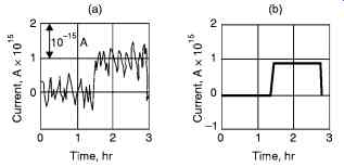
Fig. 1. Shows the effect of noise on a current waveform: (a) Experimental
strip chart recording of a 10-15 a direct current; (b) Mean of the fluctuations.
In any biological method of analysis, both instrumental and biological noise are encountered.
Example of sources of the latter include variability in the methods of application, side effects, interferences by artifact signals, and the uncontrolled effects on the rate of biological behavior as such.
Now let us discuss about the various noise generated in various components of our instruments. EEG noise which is associated with the overall behavior of cells and neurons is an example.
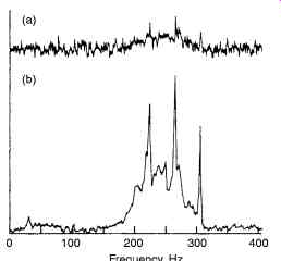
Fig. 2. Shows the effect of SNR on the NMR.
SIGNAL TO NOISE RATIO
It is apparent from Fig. 1 that the noise becomes increasingly important as its magnitude approaches that of the useful signal. Thus the signal-to-noise ratio (S/N) is a much more useful figure of merit for describing the quality of a measurement or an instrumental method than noise itself.
For a DC signal, the ultimate noise typically takes the form of the time variation of the signal about the mean as shown in Fig. 1a. Here, the noise N is conveniently defined as the standard deviation of the signal while the signal S is given by the mean. The signal to noise ratio is then reciprocal of the relative standard deviation of the measured signal. That is
S/N = mean/ standard deviation
= 1 / relative standard deviation …(1)
For an AC signal, the relationship between measured precision and S/N is less straight forward. Since most AC signals are converted into DC signal before display, this relationship will not be dealt with and the above eqn. (1) then applies.
As a rule, the visual observation of a signal become impossible when S/N is smaller than perhaps 2 or 3 as the Fig. 2 illustrates this. The upper plot is a recorded nuclear magnetic resonance spectrum for progesterone with a signal to noise ratio of approximately 4.3; in the lower plot, the ratio is 4.3. At the lower ratio, the presence of some but not all of the peaks is apparent.
NOISE SOURCES IN INSTRUMENTS
Noise is associated with each component of an instrument-that is, with the source, the transducer, the signal processor, and the read-out. Furthermore, the noise from each of these components may be of several types and arise from several sources. Thus, the noise that is finally observed is a complex composite, which usually cannot be fully characterized. Certain types of noise are recognizable, however, and a consideration of their properties is useful.
Instrumental noise can be divided into four general categories. Two, thermal or Johnson noise and shot noise, are well understood and quantitative statements can be made about the magnitude of each. It is clear that neither Johnson nor shot noise can ever be totally eliminated from an instrumental measurement. Two other types of noise are also recognizable, environmental noise or interference and flicker or 1/f noise. Their sources are not always well defined or understood.
In principle, however, they can be eliminated by appropriate design of circuitry.
JOHNSON NOISE
Johnson or thermal noise owes it source to their thermal agitation of electrons or other charge carriers in resistor, capacitor, radiation detectors, electro chemical cells and other resistive elements in an instrument. This agitation is due to motion of charge particles, is due to random and periodically created charge in-homogeneity within the conducting element. This inhomogenity in turn creates voltage fluctuations which then appear in the read out as noise. It is important to note that Johnson noise is present even in the absence of current in a resistive element.
The magnitude of Johnson noise is readily derived from thermodynamic considerations and is given by […] is the root-mean-square noise voltage lying in a frequency bandwidth of ?f Hz, k is the Boltzmann constant (1.38 × 10⁻²³ J/deg), T is the absolute temperature and R is the resistance in ohms of the resistive element.
It is important to note that Johnson noise, while dependent upon the frequency band width, is independent of frequency itself; thus, it is sometimes termed white noise by analogy to white light, which contains all visible frequencies. It is also noteworthy that Johnson noise is independent of the physical size of the resistor.
Two methods are available to reduce Johnson noise in a system: narrow the band-width and lower the temperature. The former is often applied to amplifiers and other electronic components, where filters can be used to yield narrower band-widths. Thermal noise in photo multipliers and other detectors can be attenuated by cooling. For example, lowering the temperature of the detector from room to liquid Nitrogen temperature will have the Johnson noise.
SHOT NOISE
Short noise is encountered wherever a current involves the movement of electrons or other charged particles across a junction. In the typical electronic circuit, these junctions are found at p and n interfaces; In photo cell and vacuum tubes, the junction consists of the evacuated space between the anode and cathode. The currents in such devices involve a series of quantized events, namely, the transfer of individual electrons across the junction. These events are random, however, and the rate at which they occur are thus subject to statistical fluctuations, which are described by the equation
[…]
is the root-mean-square current fluctuation associated with the average direct current I, e is the charge of the electron (- 1.6 × 10⁻¹⁹ Coulombs), and ?f is again the band-width of frequencies being considered. Like Johnson noise, shot noise has a "white" spectrum.
FLICKER NOISE
Flicker noise is characterized as having a magnitude that is inversely proportional to the frequency f of the signal being observed; it is sometimes termed 1/f (one-over-f) noise as a consequence. The causes of flicker noise are not well understood; its ubiquitous presence, however, is recognizable by its frequency dependence. Flicker noise becomes significant at frequencies lower than about 100 Hz. The long-term drift observed in dc amplifiers, meters, and galvanometers is a manifestation of flicker noise.
Environmental noise
Environmental noise is a composite of noises arising from the surroundings. Fig. 3 suggests typical sources of environmental noise.
Software Methods
With the widespread availability of micro-processors and microcomputers, many of the signal-to-noise enhancement devices described in the previous section are being replaced or supplemented by digital computer software algorithms. Among these are programs for various types of averaging, digital filtering, Fourier transformation, and correlation techniques. Generally, these procedures are applicable to non-periodic or irregular wave forms, such as an absorption spectrum, or to signals having no synchronizing or reference wave.
Some of these common software procedures are discussed briefly here.
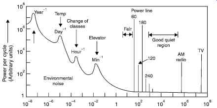
Fig. 3. Shows some sources of some environmental noises x-axis = frequency.
Ensemble Averaging
In ensemble averaging, successive sets of data (arrays), each of which adequately describes the signal wave form, are collected and summed point by point as an array in the memory of a computer (or in a series of capacitors for hardware averaging). After the collection and summation is complete, the data are averaged by dividing the sum for each point by the number of scans performed. Fig. 4 illustrates ensemble averaging of a simple absorption spectrum.
Ensemble averaging owes its effectiveness to the fact that individual noise signals Nn, insofar as they are random, tend to cancel one another. Consequently, their average N is given by a relationship,
[…]
where n is the number of arrays averaged. The signal to noise ratio of the averaged array is then given by
[…])
where Sn/n is the average signal. It should be noted that this same signal-to-noise enhancement is realized in the boxcar averaging and digital filtering, which are described in subsequent sections.
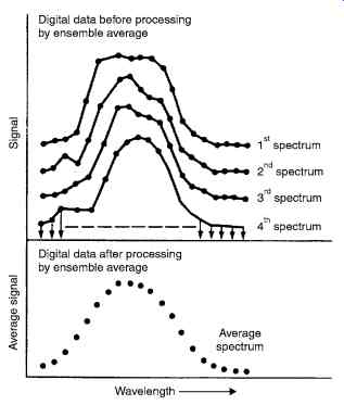
Fig. 4. Shows the Ensemble averaging of a Spectrum.
To realize the advantage of ensemble averaging and still extract all of the information available in any wave form, it is necessary to measure points at a frequency that is at least twice as great as the highest frequency component of the wave form. Much greater sampling frequencies, however, provide no additional information but include more noise. Furthermore, it is highly important to sample the wave-form reproducibly (that is, at the same point each time). For example, if the wave form is a section of ultrasound image echo, each scan of the beam must start at exactly the same position and the rate of transducer movement must be identical for each sweep. Generally, the former is realized by means of a synchronizing pulse, which is derived from the original carrier itself. The pulse then initiates the recording of the wave form.
Ensemble averaging owes its effectiveness to the fact that individual noise signals Nn, insofar as they are random, tend to cancel one another. Consequently, their average N is given by a relationship,
NN/ = n n
where n is the number of arrays averaged. The signal to noise ratio of the averaged array is then given by
[…]
where Sn/n is the average signal. It should be noted that this same signal-to-noise enhancement is realized in the boxcar averaging and digital filtering, which are described in subsequent sections.
Fig. 4. Shows the Ensemble averaging of a Spectrum.
To realize the advantage of ensemble averaging and still extract all of the information available in any wave form, it is necessary to measure points at a frequency that is at least twice as great as the highest frequency component of the wave form. Much greater sampling frequencies, however, provide no additional information but include more noise. Furthermore, it is highly important to sample the wave-form reproducibly (that is, at the same point each time). For example, if the wave form is a section of ultrasound image echo, each scan of the beam must start at exactly the same position and the rate of transducer movement must be identical for each sweep. Generally, the former is realized by means of a synchronizing pulse, which is derived from the original carrier itself. The pulse then initiates the recording of the wave form.
Ensemble averaging can produce dramatic improvements in signal-to-noise ratios. Ensemble averaging for evoked cortical potentials was considered earlier.
Ensemble averaging can be performed by either hardware or software techniques. The latter is now the more common with the signals at various points being digitized in a computer memory for subsequent processing and display.
Boxcar Averaging
Boxcar averaging is a digital procedure for smoothing irregularities in a wave form, the assumption being made that these irregularities are the consequence of noise. That is, it is assumed that the analog analytical signal varies only slowly with time and that the average of a small number of adjacent points is a better measure of the signal than any of the individual points. Fig. 5b illustrates the effect of the technique on the data plotted in Fig. 5a.The first point on the boxcar plot is the mean of points 1, 2 and 3 on the original curve; point 2 is the average of points 4, 5 and 6, and so forth. In practice 2 to 50 points are averaged to generate a final point. Most often this averaging is performed by a computer in real time, that is, as the data is being collected (in contrast to ensemble averaging, which requires storage of the data for subsequent processing).
Clearly, detail is lost by boxcar averaging, and its utility is limited for complex signals which change rapidly as a function of time. It is of considerable importance, however, for square-wave or repetitive pulsed outputs where only the average amplitude is important.
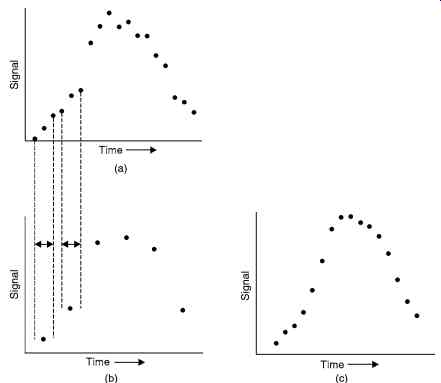
Fig. 5. Shows the effect of Boxcar averaging (a) Original Data (b) Data
after Boxcar averaging (c) Data after moving-window boxcar averaging.
Fig. 5c shows a moving-window boxcar average of the data in Fig. 5a Here, the first point is the average of original points 1, 2 and 3; the second boxcar point is an average of points 2, 3 and 4, and so forth. Here, only the first and last points are lost. The size of the boxcar again can vary over a wide range.
Digital Filtering
The moving-window, boxcar method just described is a kind of linear filtering wherein it is assumed that an approximately linear relationship exists among the points being sampled in each boxcar. More complex polynomial relationships can, however, be assumed to derive a center point for each window.
Digital filtering can also be carried by a Fourier transform procedure (see next section).
Here the original signal, which varies as a function of time (a time-domain signal), is converted to a frequency-domain signal in which the independent variable is now frequency rather than time.
This transformation, is accomplished mathematically on a digital computer by a Fourier transform procedure. The frequency signal is then multiplied by the frequency response of a digital filter, which has the effect of removing a certain frequency region of the transformed signal. The filtered time-domain signal is then recovered by an inverse Fourier transform.
Correlation
Correlation methods are beginning to find application for the processing of data from medical instruments. These procedures provide powerful tools for performing such tasks as extracting signals that appear to be hopelessly lost in noise, smoothing noisy data, comparing a diagnostic (ecg signal) with a stored previous signal of the same patient, and resolving overlapping or unresolved peaks in spectroscopy and chromatography. Correlation methods are based upon complex mathematical data manipulation that can only be carried out conveniently by means of a digital computer.
Correlation (k) = XY mn k n
?0 N where X is correlated to Y. and N = total number of samples. Cor. (k) is signal giving the correlation.
FOURIER TRANSFORMS
Wavelets and wavelet transforms are a relatively new topic in signal processing. Their development and, in particular, their application remains an active area of research.
Time-frequency signal analysis and the STFT In signal analysis, few, if any, tools are as universal as the Fourier transform. It is used as the keystone of modern signal processing. The Fourier transform and its inverse are defined as follows:
[…]
where F(?) is the Fourier transform of the signal f(t).
Using the identity.
[…]
the inverse transform can be described in terms of sine and cosine functions rather than complex exponentials:
[…]
From this it can be seen that the Fourier transform F(?) of a signal is a function describing the contribution of sines and cosines to the construction of the original time domain signal.
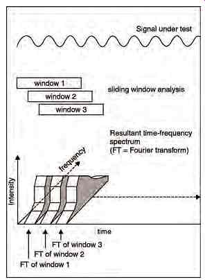
Fig. 6. Shows STFT sliding window analysis.
Software Methods
With the widespread availability of micro-processors and microcomputers, many of the signal-to-noise enhancement devices described in the previous section are being replaced or supplemented by digital computer software algorithms. Among these are programs for various types of averaging, digital filtering, Fourier transformation, and correlation techniques. Generally, these procedures are applicable to non-periodic or irregular wave forms, such as an absorption spectrum, or to signals having no synchronizing or reference wave.
Some of these common software procedures are discussed briefly here.
Fig. 6 shows the STFT sliding window analysis.
The time independence of the basis functions of the Fourier transform results in a signal description purely the frequency domain. The description of a signal as either a function of time or as a spectrum of frequency components contradicts our everyday experiences. The human auditory system relies upon both time and frequency parameters to identify and describe sounds.
For the analysis of non-stationary signals a function is required that transforms a signal into a joint time-frequency domain. Such a description can be achieved using the well known STFT, which is an extension to the classical Fourier transform as defined by Gabor:
[…]
This function can be described as the Fourier transform of the signals s(t), previously windowed by- the function g(t) around time t. As the window function is shifted in time over the whole signal and consecutive overlapped transforms are performed, a description of the evolution of signal spectrum with time is achieved. This method assumes signal is stationary effectively over the limited window g(t). If the window is relatively short, this assumption of local stationary is often valid. Eqn. (8) can be described diagrammatically as shown in Fig. 6. As the window function g(t) is shifted in time, repeated Fourier transforms chronologically, on a common frequency axis, it provides a time-frequency description of the signal which is commonly called the signal spectrogram. Such displays are considered in ultrasound Doppler cardiography.
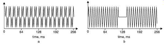
Fig. 7. Shows a test signals (a) 64 Hz and (b) 128 Hz with a 64 sample
gate.
Fig. 7 shows two simple test signals, both 256 ms long and sampled at a rate of 2000 samples per second. The test signal in Fig. 7a comprises two sinusoids of equal amplitude, one at 64 Hz and one at 192 Hz. The second test signal, in Fig. 7b, contains a single sinusoid with a 64-sample gap, during which the signal is 'switched off'. Fig. 7a shows the STFT of the test signal in Fig. 8a using a relatively long window length of 128 samples and Fig. 8b shows the STFT of the same signal with a shorter 32-sample window. The longer window length results in better frequency resolution and, as can be seen in Fig. 8a, the two sinusoids are clearly re solved. The shorter window length results in reduced frequency resolution and this analysis, shown in Fig.8b, fails to resolve the two sinusoidal components. Fig. 9 clearly demonstrates how transform window length affects resolution in frequency.
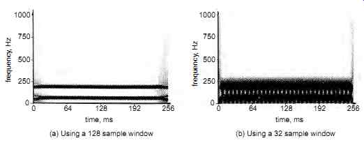
Fig. 8. Shows STFT of the TEST signal (a) using different windows. (a)
Using a 128 sample window (b) Using a 32 sample window
Fig. 9 shows the results of transforming the test signal in Fig. 7b, again using a long 128-sample window and a short 32-sample window. As would be expected, applying the longer 128-sample analysis ( Fig. 9a) fails to resolve the signal gap but the short 32-sample analysis (Fig. 9b) quite clearly resolves the position and length of the gap. Fig. 8 and Fig. 9 together illustrate the joint time and frequency resolution limitations of the STFT implied by the uncertainty principle.
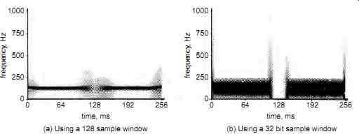
Fig. 9. Shows STFT of the signal (b). (a) Using a 128 sample window (b)
Using a 32 bit sample window
In most bio signals, high frequency resolution characteristics are not required.
THE WAVELET TRANSFORM
Previously, the STFT (Eqn.8) has been analyzed as the Fourier transform of the windowed signal s(t) . g(t-t), but it is just as valid to describe this function as the decomposition of the signal s(t) into the windowed basis function g(t-t) exp(- j?t). The term 'basis functions', refers to a complete set of functions that can, when combined as a weighted sum, be used to construct a given signal.
In the case of the STFT these basis functions are complex sinusoids, exp(- j?t), windowed by the function g(t) centered around t.
It is possible to write a general equation for the STFT in terms of basis functions kt,? (t)and signal s(t) as an inner product:
STFT (t, ?) = ? s(t) kt, ? (t) dt …(9)
For the STFT, basis functions in Eqn.(9) can be represented by kt, ? (t)) = g(t) e-j?t
Fig. 10a shows the real part of three such functions to demonstrate the shape of typical STFT basis functions. These windowed basis functions are distinguished by their position in time t and their frequency. By mapping the signal onto these basis functions, a time-frequency description of the signal is generated.
The WT can also be described in terms of its basis functions, known as wavelets, using Eqn. (9). In the case of the WT, the frequency variable v is replaced by the scale variable a and generally the time-shift variable t is represented by b. The wavelets are represented by
[…]
Substituting this description into Eqn. 9 gives the definition for the continuous wavelet transform (CWT):
[…]
From the above Eqn.(10), it can be seen that the WT performs a decomposition of the signal s(t) into a weighted set of scaled wavelet functions h(t). In general the wavelet h(t) is a complex valued function; Fig. 10b shows the real part of the Morlet wavelet at three different levels of scale. Comparing the two sets of basis functions in Fig. 10, it can be seen that the wavelets are all scaled versions of a common 'mother wavelet' whereas the basis functions of the STFT are windowed sinusoids.
(a) Short-Time Fourier Transform
(b) Wavelet Transform
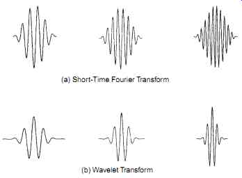
Fig. 10. Shows a typical basis functions
Due to the scaling shown in Fig. 10b, wavelets at high frequencies are of limited duration and wavelets at low frequencies are relatively longer in duration.
These variable window length characteristics are obviously suited to the analysis of signals containing short high-frequency components, and extended low frequency components which is often the case for signals encountered in practice.
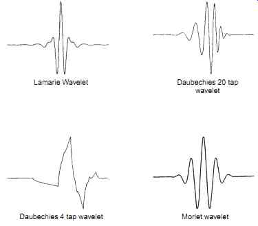
Fig. 11. Shows common wavelets used. Lamarie Wavelet Daubechies 20 tap
wavelet; Daubechies 4 tap wavelet Morlet wavelet
Fig. 11 shows a number of commonly used wavelets.
The CWT as a time-scale transform has three dimensions. The three dimensions are rep resented on a log (a),b half-plane. The log (a) axis (scale) faces downwards and b- axis (time-shift) faces to the right. The respective intensity of the transform at points in the log(a), b half-plane is represented by grey level intensity. These conventions allow a standard plot of time evaluation from left to right and decreasing frequency from top to bottom, The phase is not displayed if the transform modulus drops below a predetermined cutoff value.
By employing scaled window functions, the WT does not overcome the uncertainty principle, but by employing variable window lengths, and hence variable resolution, an increase in performance may be achieved. Fig. 8 and Fig. 9 demonstrated the resolution limitations imposed upon the STFT by the uncertainty principle. Fig. 12 shows the magnitude and phase plots generated by applying the WT to the two test signals of Fig. 7. It can be seen from Fig. 12 that in both test cases the WT has clearly separated the signal components.
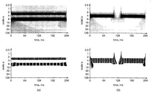
Fig. 12. Shows (a) Magnitude and Phase plot of the two sinusoid (b) Magnitude
and phase plot of the wavelet transform of a sinusoid with gap test signal.
Localization of signal discontinuities by the V-shape in Fig. 12b is an important characteristic of the WT that can be used in signal interpretation.
Many algorithms have been developed by the researchers for calculating WTs. One such algorithm is based upon the fast Fourier transform (FFT), By analyzing the CWT in the Fourier domain the basic convolution operation of the CWT can be achieved via simple multiplication operations. Writing the CWT in the Fourier domain gives
F{CWT (b, a)} = (1/va) H*(?/a) S(?) …(11)
...where F{CWT(b, a)} is the Fourier transform of the continuous wavelet transform, H*(w) is the Fourier transform of the wavelet and S(w) is the Fourier transform of the input signal. This equation can be used as the basis of an FFT-based fast wavelet transform. Eqn. (11) can be represented graphically as shown in Fig. 13.
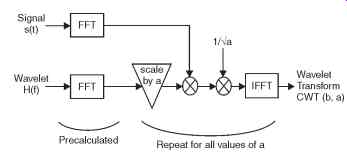
Fig. 13. Showing the Block Diagram of the FFT based Fast Wavelet transform.
If the Morlet wavelet is adopted:
h(t) = exp( j ?0 t) . exp(- t2/2) …(12)
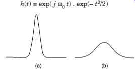
Fig. 14. Shows magnitude of the Morlet wavelet (a) low value (b) increased
scale value.
WAVELET TRANSFORM OF A TYPICAL ECG
The example of the application of the WT is the transformation of an electrocardiograph (ECG) trace. A typical ECG trace is shown in Fig. 15a. The magnitude and phase plots resulting from the transformation of this signal, again using the Morlet wavelet, are shown in Figs. 15b and 15c, respectively. The magnitude plot shows a large degree of spreading over the time-scale plane. This spreading may be explained in two ways. Localization in the time-scale plane occurs when the signal and wavelet show a high degree of similarity. Comparing the ECG trace and the Morlet wavelet in Fig. 11, it can be seen that the two waveforms show little, if any, similarity.
Hence, localization of the transform is not expected.
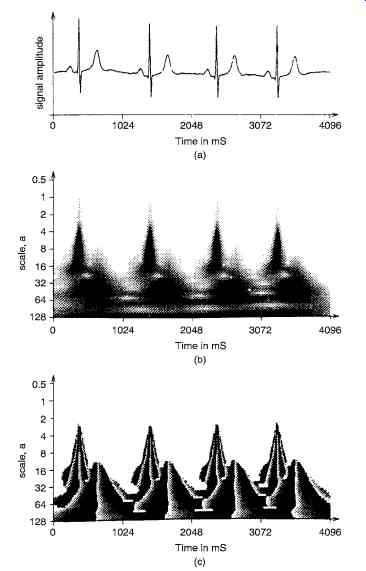
Fig. 15. Shows the wavelet transform of a typical ECG : (a) Input signal
(b) Transform magnitude (c) Transform phase.
The WT is particularly apt at highlighting discontinuities. Due to the sudden depolarization and repolarization of cardiac tissue, the ECG contains a number of distinct peaks. It can be seen from the WT of the ECG that these peaks are highlighted as upturned V's, which become increasingly spread in time as scale increases. Although the impulsive nature of the ECG trace results in a spread transform at high scale values, it can be seen that at low values of scale, distinct time localization occurs. This localization characteristic can be used to pinpoint the significant peaks of the ECG trace. The position of significant complexes and peaks in the ECG waveform is an important diagnostic tool in detecting pathological conditions relating to the muscular and electrical aspects of tissue of the heart. These results point to the application of the WT to the automatic identification and characterization of such pathological conditions.
TIME VARYING FILTERING IN EVOKED POTENTIALS
New Signal Processing technique
Evoked potentials (EPs) or event related potentials (ERPS) are brain responses which occur along with the electroencephalogram (EEG) to specific activation of sensory pathways. Such responses are commonly used for the clinical examination of neural pathways of perception and for better understanding of the human behavior and the functioning of the central nervous system (CNS). Abnormal EPS are often indicator of nervous system illness or injury. Abnormalities can be in the form of slow impulse propagation velocities or an irregular wave shape measured on the scalp. For most applications, measurements are made by means of electrode attached to the scalp.
The ERPs having an amplitude in the range of a fraction of a microvolt to a few millivolts, are buried in the background EEG activity. The SNR is very small, of the order of - 10dB or less. It is this small SNR that makes evoked potential signal estimation very difficult.
Averaging a number of trials, also called ensemble averaging, remains one of the most popular techniques to extract the ERP signal from the ongoing, seemingly random background EEG noise. Depending on the SNR, the number of measurements needed for averaging to obtain a reliable estimate ranges from a few dozen (for visual evoked potentials, VEP) to a few thousand (for brainstem auditory evoked potentials, BAEP). The inherent assumptions in averaging are, that the signal is deterministic and does not change from stimulus to stimulus and the EEG noise is stationary with zero mean and is uncorrelated with the signal and from trial to trial. However, statistical tests have shown possible trial to trial temporal and morphological variability of event related processes. Different techniques have been proposed for the EP signal estimation on distinctly different assumptions regarding the signal noise or the signal generating processes.
Prev. | Next