AMAZON multi-meters discounts AMAZON oscilloscope discounts
WIENER FILTER AND ITS APPLICATIONS TO EVOKED POTENTIALS
Wiener original theory solves the problem of optimal signal estimation in the presence of additive noise, with known power density spectra of signal and noise. His optimal filter function is given by,
[…]
where H(f) is the filter transfer function and Gss (f) and Gnn(f) are the known power density spectra of signal and noise. This filter, when applied to the observed signal, leads to an optimal estimate of the signal in the mean square error sense. Wiener's theory assumes both the signal and the noise to be random, stationary, ergodic processes with known correlation functions. The application of the evoked potentials is done using the estimated power density spectra of signal and noise.
A Posteriori WIENER FILTER
Wiener theory for filtering noisy signals has been used in the study of EPs, by many researchers.
De Weerd et al have done an exhaustive study of the effectiveness of Wiener filtering in improving the SNR of average evoked potentials. The idea behind a posteriori filtering is to improve the estimation of the real signal, as obtained after ensemble averaging, still further by a linear filtering procedure. The appropriate filter transfer function is computed form the estimates of the underlying spectra of signal and noise. A posteriori Wiener filtering is suggested to obtain an improved signal estimate beyond averaging in the case of evoked potentials by De Weerd et al.
The central idea of a posteriori Wiener filtering is that an averaged signal that is still contaminated with noise could be improved using a posterior estimated power density spectra of the signal and noise. However, with decreasing signal to noise power density ratio (SNPNR), the transfer function suffers from larger bias and variance due to the variability in the spectra computed.
Considering a fixed latency evoked potential model, […] s(t) represents the signal, ni (t) noise, N is the number of stimulus presentation and T is the duration of evoked potential.
Responses which show considerable trial to trial variability may be denoted by variable latency evoked potential model, […] represents the random variable. The following matter, however assumes the fixed latency model.
If the power density spectra of signal and noise were known a priori, the optimum Wiener filter transfer function for use on the ensemble average is
H(f) = Gss
[…] represent known power density spectra of the signal and the noise. In practice, however, these spectra are unknown but can be estimated from the ensemble as suggested. In this, a spectrum of the ensemble average in which the noise power is reduced by a factor proportional to the number of ensemble elements is taken as the PSD of the signal and an average of the spectra of individual ensemble elements, in which the noise power is not reduced, is taken as the PSD of the noise. If the PSD of the ensemble average XN(t) be denoted by fxxn(?), it implies that the transfer function itself becomes an estimate.
By alternate averaging, (i.e.) by alternate addition and subtraction of ensemble elements, the signal averages out, and the power density spectrum of the alternate average XN(t) is an estimate of the power density spectrum of the noise reduced by a factor N. The principal advantage of alternate averaging is that due to the alternate addition and subtraction and successive ensemble elements, such inhomogenities tend to average out, which implies that the corresponding estimator becomes less biased. Instead of using the full ensemble for calculation of the alternate average and its corresponding spectrum, sub-ensemble averaging is preferred because the inhomgenities caused by trends, slow amplitude modulations of the signal or a slow changing character of the background etc. can be taken care.
The methods for separation of signal and noise spectra as discussed above are applicable when dealing with an ensemble in which each element is conceptually composed of an invariant signal and an additive stationary noise component, uncorrelated with this signal.
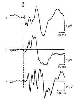
Fig. 16. Shows a typical examples of evoked potential from the human brain.
(a) Somatosensory evoked potential (b) Visual evoked potential (c) brainstem auditory evoked potential.
SIGNAL PROCESSING IN HEART-RATE VARIABILITY-LINEAR ANALYSIS
The heart rate variability (HRV) signal derives its significance from the facts that (i) it provides a noninvasive window to study the autonomic nervous system (ANS), (ii) it is altered in different disease states and (iii) changes in ANS activity may be important indicators of patient outcome.
HRV analysis concerns with the systematic, quantitative study of the fluctuations in the heart rate.
The ECG is sampled at a sufficiently high rate (usually 500 Hz) to determine the time locations of the R waves at the accuracies needed for the analysis. The R waves are detected using a suitable algorithm, and the so-called normal-to-normal (NN) intervals (that is, all intervals between adjacent QRS complexes resulting from sinus node de-polarizations) are determined. From this R-R interval series, several time domain descriptors of the variability are computed.
SPECTRAL DOMAIN ANALYSIS
However, a simple linear interpolation gives results as good. From this uniform interval HR series, the mean is then removed. Either non-parametric (FFT) or parametric (usually, Autoregressive) spectrum of this HRV signal is then obtained. Fig. 17 shows sample HRV spectra for supine and standing postures of a subject. By means of studies where the autonomic components were selectively blocked, they have identified that different frequency components in the HRV spectrum have been contributed by different aspects of the physiological system. Based on the results of these studies, the spectrum is divided into three distinct bands, namely, the very low frequency band (VLF, frequency range 0.01-0.04 Hz), the low frequency band (LF, 0.04-0.15 Hz) and high frequency band (HF, 0.15-0.40 Hz). Drugs such as atropine are selective parasympathetic blocking agents and by employing them on normal individuals, the HF peak has been identified to be correlated to the respiratory driven vagal (parasympathetic) efferent input to the sinus node. Similarly, propanolol is a strong sympathetic receptor blocker, with the help of which, the LF band (definitely during standing position) is known to represent the sympathetic vagal drive. The VLF band is supposed to be linked to the thermoregulatory system, though the evidences are inconclusive. Accordingly, the absolute power (in millisecond squared) in all the 3 frequency bands and ratios of HF and LF to total HRV power are calculated. A ratio of the energies in the LF and HF bands is currently being accepted as representing sympatho-vagal balance. LF norm and HF norm are the LF and HF powers in normalized units (i.e. LF or HF/ (total power-VLF) * 100, where total power is defined as the power in the frequency band < 0.4 Hz.
The representation of LF and HF in normalized units emphasizes the controlled and balanced behavior of the two branches of the ANS and also tends to minimize the effect of the changes in total power on the values of LF and HF components.
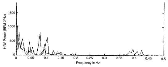
Fig. 17. Shows the power spectrum of HRV (I-Supine; II standing).
Though most studies have analyzed HRV samples, a few investigators [Murata] have directly obtained the power spectrum of the R-R interval series, ignoring the fact that the latter is a non uniformly sampled data. These results are not always directly comparable to those obtained from the HRV series.
CLINICAL APPLICATIONS
The anatomic location of the autonomic nervous system (ANS) renders it inaccessible to direct physiological testing. The study of HRV Power Spectra is gaining acceptance as a non-invasive method for identifying the role of the ANS in regulating cardiac function. HRV decreases with age and this factor must be kept in mind while interpreting the results of any study. It may be possible to roughly normalize the data with respect to age. HRV analysis being a field of current research, the possible clinical applications are increasing. The following are some of the potential clinical uses already identified.
1. Decreased HRV is predictor and adverse outcome after a myocardial infarction. Low HRV for such patients means automatic unbalance which can be fatal.
2. Side effects of drugs in psychiatric patients causes HRV reduction. This is an extension of the Z-transform in sampled data ( discrete ) analysis of bio-signal.
CHIRP-z-TRANSFORM
Fig. 18 shows the Z-plane with a spiral trajectory drawn on it. The spiral trajectory is marked out at angular intervals f corresponding to the M frequencies (values of ?) for which the z-transform has to be evaluated.
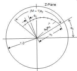
Fig. 18. Shows Chirp-z-transform over trajectory on the z-plane.
Fig. 19 shows Chirp z transform over a trajectory on the Z plane
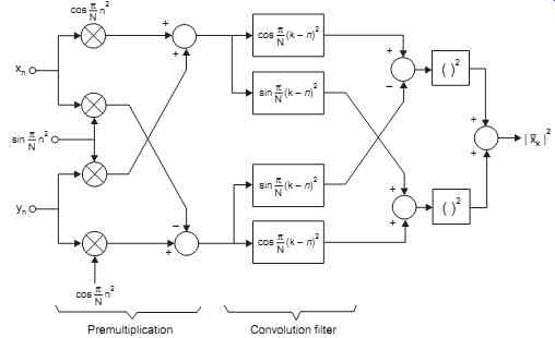
Fig. 19. Shows the phase quadrature scheme of doppler signal excitation.
The spiral trajectory is defined in the following equations:
[...]
The chirp-z algorithm provides an efficient method for finding the transform X(Zk) given by [...]
where the summations extend from 0 to M-1
Using the equation 2kn = k2
+ n2
- (k - n) 2, this expression is manipulated algebraically to give a convolution of two sequences with scaling as follows:
[...]
This is the summation equivalent to g(n)*h(n)
Therefore X(zk) = [1/h(k)] S g(n)h(k - n)
The summation is required convolution operation and the result X(zk) is a sequence, in principle of indefinite length which we truncate to give our required M output samples. It is interesting to note that h(n) is a complex exponential sequence with a linear increase in frequency.
h(n) = (W0 exp (- jf0)n2 2/
which may be rewritten as h(n) = (W0 exp (- jn (f0 n/2)) The brackets (f0 n/2) can be regarded as a frequency which steadily increases with time (n); such a signal is known as a chirp and it is from this that the operation gets its name. The convolution is carried out rapidly be means of an FFT routine and appropriate scaling is applied to the final result. The computations are as depicted in Fig. 19.
The convolutions are performed using CCD ICs (R6502) in the ultrasound machines.
Fig. 19 shows chirp-z transform Computation of spectral power density.
HILBERT TRANSFORM
Though the Hilbert transform is a very important component in any analytic signal comprising a real part and quadrature part), its use is noted to be rather not prominent. However, this was useful in an application to Doppler echo-cardiography.
The Hilbert transform of a real signal is the all - pass filtered output with no magnitude change but a fixed - p/2 phase change for positive frequencies, and a + p/2 phase change for negative frequencies. The transfer function of the transform is shown in Fig. 20.
The Hilbert transform relates the tow components of a complex signal ...
Thus, one component is the transform of the other, if the signal satisfies Cauchy-Reimann conditions.
In work with signals from ultrasound machines, this transform is useful to relate the two I and Q components of the synchronously detected signal.
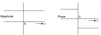
Fig. 20. Shows the Hilbert transform transfer function.
A program for quickly evaluating the Hilbert transform of a large set of data samples was written using a matrix formulation of relations. The Hilbert transform of a discrete sequence xv is obtained by:
where L = (N/2) - 1 when N is even and (N - 1)/2 when N is odd.
The above Hilbert transformed sequence can be put in matrix notation as :
[…]
Since the rows are circulant, by evaluating one row and keeping it stored, it was possible to generate the other rows by shift operations; the output vector is thus easily obtained as the product of sum. This operation can be the implemented very rapidly in DSP hardware and could show the waveforms as quickly as the machine shows the spectrogram.
ECG DATA COMPRESSION
AZTEC
The amplitude zone Epoch Coding (AZTEC) data-reduction algorithm has become an accepted from of data reduction for ECG monitors, and data bases recently. AZTEC takes raw ECG data and produces short lines and slopes. Fig. 21 shows how this is done.
Horizontal lines As the monitor samples the ECG, the first sample is set equal to the initial conditions, one of Vmax and Vmin. The next sample is compared to Vmax and Vmin. If the sample is greater than Vmax, then Vmax is made equal to the sample value. Conversely, if the sample is less than Vmin, then Vmin is made equal to the value of the sample. This process is repeated until either the difference between Vmax and Vmin is greater than a predetermined threshold, Vthresh, or more than 50 samples have been gathered. Either event produces a line. To store the line, first the number of samples examined minus one is saved at T1 ( time or length of line). Then the values of Vmax and Vmin, previous to the present sample, are averaged and set to V1, which is saved (i.e., the value of the line, V1 = (Vmax + Vmin)/2 at time (t - 1).
Vmax and Vmin are then set equal to the present sample and the process is continued. This is the first part of AZTEC algorithm and is called zero-order interpolation (ZOI). This ZOI produces lines of zero slope. The first value saved is the length of the line, while the second value is the amplitude of the line.
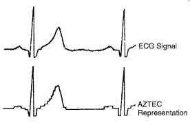
Fig. 21. Shows the original data and the output.
First, the value of the line is assigned to Vslope1. Second, the length of the line is assigned to Tslope1 ( time or length of the slope1). This direction of the slope (+ or -) is also recorded. When the next line is produced, AZTEC determines whether or not the slope data should be updated or terminated. Then, the slope parameters are determined and saved. If the slope was terminated by a change in direction and / or the terminating line length is greater than 2, the amplitude of that line is saved, then the length of the line, and finally the amplitude of the lines are saved again.
AZTEC's data reduction is not constant. The reduction is frequently as great as 100/1000 or more, depending upon the nature of the signal itself and the value of the empirically determined threshold.
Although AZTEC produces a recognizable ECG signal, the step like quantization is unfamiliar to most nurses and physicians. Therefore, a curve smoothing algorithm to process the AZTEC data produces a more acceptable output for the nurses and physicians.
Parabolic fitting provides a smooth - curve approximation to each set of seven points in the original waveform.
P0 = 1/2T (- 2ak-3 + 3ak-2 + 6ak-1 + 7ak + 6ak+1 + 3ak+2 - 2ak+ 3) where P0 is the new data point and ak± n the original data points (AZTEC), and k ± n defines the time relationship.
For R wave detections, scanning through the data to look for a slope greater than 1/3 of the height of the normal QRS of the patient, is done. If no such R wave is found, the trial is done with a slope of 1/6 of the height. When no R wave is detected in a time of twice the R-R interval, a "missing beat" is indicated. If more than one R-wave is noted, the higher amplitude is taken as R wave, the other can be a P wave and R-R interval is used for calculating the sinus rhythm.
Therefore, we can take advantage of AZTEC's superior data compression while retaining the clinical information content of the ECG for diagnostic purposes.
AZTEC Program for ECG compression
The program (in Basic) given below is in 2 parts. First, for testing, it generates an ECG file of data points. Second, it compresses this file. The program also displays the two signals-the actual data plotted, and the points selected on the compression by AZTEC.
When using with data collected clinically, the first part of the program is removed; but the ECG clinical data must be available as a file {a: ecgfile}. It is possible to generate short ecg file from clinical data with a PC-based data acquisition card or via the printer port. The data for up to 5 or 6 ECGs are enough for the file.
Then, the second part of the program ( starting from str = 1 instruction) is run to generate the compressed file, which is also printed out. The maximum number of compressed data in this program is 128, but it can be altered.
Please note how the points chosen on the AZTEC algorithm, when joined, give the ECG of almost the same shape as the original data.
Figure above shows how the data of the compressed format merges almost with the actual data in the above AZTEC program.
The turning point algorithm
This is another algorithm. This reduces the sample points to half the original. Suppose 200 points were taken for one e.c.g. wave, it will become 100.
The first point sampled X0, is called reference. The next two are X1, X2. Since among these three points, there can be only one of the following changes, the change that is relevant is shown
and selected as the point for compressed data. Thus, if X0 - X1 - X2 is a progressive rise, the X2 point alone is selected.
The next 2 points are chosen, of which one is selected and so on goes the entire data compression.
Since, a program cannot recognize the figure shown here, the slopes of the point pair which are X2 - X1 and X1 - X0 are compared as positive or negative. The product is taken. X1 is saved if it is negative, while X2 is saved when it is positive or zero.
[...]
Choose X2 A second application of the algorithm to the compressed data is sometimes done but it may not be good enough.
Showing method of choice of compressed point in Turning point algorithm.
ECG CLASSIFICATIONS
Fig. 22 shows how a computer classification of grade for an ECG would be (of course, all clinical ECGs are grade - 1 only).
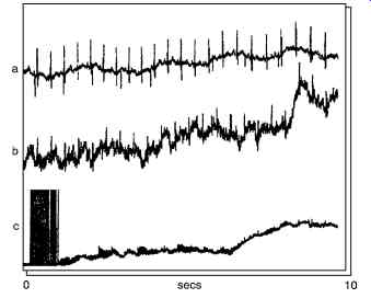
Fig. 22
An FIR or IIR bandpass digital filter may be used to pre- process the raw ECG before QRS detection. We prefer the use of FIR as an IIR filter of a high order, (for example eighth order);
sometimes rings when excited by the narrow width QRS complexes which may complicate the precise location of the R wave. The filter specifications used in the study are as follows.
AZTEC
Filter length 75
Sampling frequency 500 Hz
Stopbands 0-1Hz, 47-250 Hz
Passband 9 - 39
Pass band ripple 0.5 dB
Stopband attenuation 30 dB
Figs. 14 a to c show the filtered ECG data. Compared with the corresponding unfiltered raw data, figures a-c, the baselines shifts as well as the high frequency noise have been reduced in the filtered data (ignoring the transients and the initial transients in the filtered data). In the grade - 3 data, the ADC error appears as a burst which no doubt will confound most QRS detection algorithms.
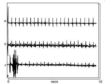
Fig. 23
Bandpass filtering on ECG
From the spectral analysis of the various signal components in the ECG signal, a filter can be designed which effectively selects the QRS complex from the ECG. Fig. 24 shows a plot of the signal-to-noise ratio (SNR) as a function of frequency. The study of the power spectra of the ECG signal, QRS complex, and other noises also revealed that a maximum SNR value is obtained for a bandpass filter with a center frequency of 17 Hz and a Q of 3.
Fig. 24. Plots of the signal-to-noise ratio (SNR) of the QRS complex referenced to all other signal noise based on 3875 heart beats. The optional bandpass filter for a cardio-tachometer maximizes the SNR.
Two Pole recursive filter
A simple two-pole recursive filter can be implemented in the C language to bandpass the ECG signal. The difference equation for the filter is
[...])
Two Pole Recursive (int data)
[...]
This filter design assumes that the ECG signal is sampled at 500 samples/s.
It is to be noted that in this code, the coefficients 1.87635 and 0.9216 are calculated easily by 1.875 = 1 + ½ + ¼ + 1/8
... and 0.9219 = ½ + ¼ + 1/8 + 1/32 + 1/64
... so that right shift operations are useful.
INTEGER FILTER
QRS detectors for cardio-tachometer applications frequently bandpass the ECG signal using a center frequency of 17Hz. The denominator of the general form of the transfer function allows for poles at 60°, 90° and 120°, and these correspond to center frequencies of a bandpass filter of T/6, T/4, and T/3 Hz, respectively. The desired center frequency can thus be obtained by choosing an appropriate sampling frequency.
A useful filter for QRS detection is based on the following transfer function:
H(z) = (1 - z-12) 2/(1 - z-1 + z-2) 2
This filter has 24 zeros at 12 different frequencies on the unit circle with poles at ± 60°. The ECG signal is sampled at 200 sps, and then the turning point algorithm is used to reduce the sampling rate to 100 sps. The center frequency is at 16.67 Hz and the nominal bandwidth is ± 8.3 Hz.
The difference equation to implement this transfer function is
[…]
QRS Template
Most QRS detection methods rely on the availability of a representative QRS template against which the incoming ECG signal is compared. The template may be generated from raw ECG data by detecting and averaging several good QRS complexes. This may be done automatically or semi manually by visually examining a grade 1 ECG record and identifying good, unambiguous ECG complexes. The R waves are then synchronized and the QRS complexes averaged. A fixed QRS template may be used to detect v complexes or a new one may be generated at the start of each ECG record. An example of a QRS template obtained by averaging 69 QRS complexes in grade 1 data and then taking 31 samples (15 samples on either side of the R wave) of the averaged QRS complexes is shown in Fig. 25.
Sample Index
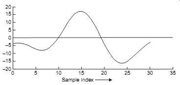
Fig. 25. An example of a QRS complex template. This is obtained by averaging
over 69 QRS complexes in a grade 1 ECG, with the R-waves synchronized.
The QRS complexes were detected with a threshold level of 13.
In a study, templates of various lengths were tried. Typically, the length of the template, N, is between 11 and 31 samples, that is a width of between about 20 ms and 60 ms at a sampling rate of 500 samples s-1. Good results are obtained with two templates of lengths 11 and 31 samples.
QRS detection methods
A general block diagram of the QRS detection process is given in Fig. 26. The raw ECG data is first pre-processed to reduce the effects of noise. The pre-processed data samples are fed into a buffer one data point at a time. For each new data point fed into the buffer, the oldest data point is removed and the content of the buffer compared with a QRS template in the QRS detector.
The output of the QRS detector is then thresholded. If this output exceeds the threshold value then a QRS is said to have occurred. Two conventional QRS detection methods are compared now, selected on the basis that they are either in practical use or potentially of practical use.
Many other QRS detection methods exist.
The methods are:
1. average magnitude cross-difference(AMCD) (Lindecrantz) currently used in a new fetal monitor described in Lindecrantz; and
2. matched filtering, which is a common QRS detection method and has been investigated by a number of workers.
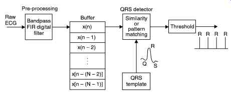
Fig. 26. Concepts of QRS complex detection from raw ECG.
Average magnitude cross-difference
In this method blocks of pre-processed data are compared against a template QRS complex as described above. The differences between corresponding samples in ECG and the template are computed by waveform subtraction. The sum, y(i), of the absolute values of the differences is then computed:
where xt ...
(k) are samples of the template QRS complex, x(k + i) are samples of the ECG signal, N is the length of the template, and I is the time shift parameter. xt
is the mean value of the QRS template, and xi [...] the mean value of the ith data block for the ECG signal given by [...]
When the ECG signal and QRS template are very similar in shape, that is in the neighborhood of a QRS complex, the AMCD value, y(i), becomes a minimum (theoretically zero).
Fig. 27. In simple template matching, the incoming signal is subtracted, point by point, from the QRS template. If the two waveforms are perfectly aligned, the subtraction results in a zero value.
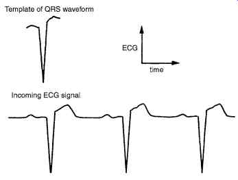
Fig. 27 shows the method used in simple template matching.
Digital matched filtering
Matched filtering is commonly used to detect time recurring signals buried in noise. The main underlying assumptions in this method are that the signal is time limited and has a known waveshape. The problem then is to determine its time of occurrence. The impulse response of a digital matched filter, h(k), is the time-reversed replica of the signal to be detected. Thus in our case, if xt
(k) is the QRS template then the coefficients of the matched filter are given by h(k) = xt (N - k - 1), k = 0, 1, . . . , N - 1 ...(14.2)
The digital matched filter can be represented as an FIR filter with the usual transverse structure, with the output and the input of the filter related as [...] where x(i) are the samples of the input ECG signal, xt
[...] (k) are the samples of the QRS template, N
[...] is the filter length, h(k) are matched filter coefficients, and i is the time shift index. It is evident that when the template and the QRS complex coincide, the output of the matched filter will be a maximum. Thus by searching the output of the matched filter for a value above a threshold the occurrence of the QRS can be tested.
Performance measure for QRS detection
To evaluate and compare the algorithms requires a measure of performance. Following Azevedo and Longoni define the performance measure as
(Total number of R waves - number of misses - number of false detections)
100% Total number of actual R waves
For a given ECG record, the performance measure attains a value of 100% only if all the R waves in the record are correctly detected, with no misses (undetected R waves) and no false detections (false alarms). For a given QRS detection method, the number of misses or false detections can be determined by comparing, visually, the output of the detector and the pre-processed ECG.
Overall, the AMCD and matched filtering methods are nearly same in terms of their performance. With suitable threshold level, both methods attained the following performances:
Automata-based template matching
Fig. 28 shows the set of tokens that would represent a normal ECG. Then this set of tokens is input to the finite state automaton defined in Fig. 29. The finite state automaton is essentially a state-transition diagram that can be implemented with IF…… THEN control statements available in most programming languages. The sequence of tokens is fed into the automaton. For example, a sequence of tokens such as zero, normpup, normdown, and normup would result in the automaton signaling a normal classification for the ECG.
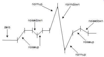
Fig. 28. Reduction of an ECG signal to tokens.
The sequence of tokens must be derived from the ECG signal data. This is done by forming a sequence of the differences of the input data.
This QRS detector first 'learns' about the R-wave, where the program approximately determines the peak magnitude of a normal QRS complex. Then the algorithm detects a normal QRS complex each time there is a deflection in the waveform with a magnitude greater than half of the previously determined peak. The algorithm now teaches the finite state automaton the sequence of tokens that make up a normal QRS complex. The number and sum values for a normal QRS complex are now set to a certain range of their respective values in the QRS complex detected.
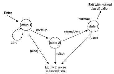
Fig. 29. State-transition diagram for a simple automaton detecting only
normal QRS complexes and noise. The state transition (else) refers to any
other token not labeled on a state transition leaving a particular false.
The program can now assign a waveform token to each of the groups formed previously, based on the values of the number and the sum in each group of differences. For example, if a particular group of differences has a sum and number value in the ranges (determined in the learning phase) of a QRS upward or downward deflection, then a normup or normdown token is generated for those group of differences. If the number and sum values do not fall in this range, then a noise-up or noise-down token is generated. A zero token is generated if the sum for a group of differences is zero. Thus, the algorithm reduces the ECG signal data into a sequence of tokens, which can be fed to the finite state automation for QRS detection.
Filter based QRS Detector
Fig. 30 shows the filter stages of the QRS detector. z(n) is the time-averaged signal y(n) is the band passed ECG, and x(n) is the derivative of the ECG.
A bandpass filter picks up the predominant QRS energy centered at 10Hz, attenuates the low frequencies characteristic of P, T waves and baseline drift, and also attenuates the higher frequencies. The next processing step is differentiation, a standard technique for finding the high slopes that normally distinguish the QRS complexes from other parts of ECG wave.
Next is a nonlinear transformation that consists of point-by-point squaring of the signal samples. This transformation serves to make all the data positive prior to subsequent integration, and also enhances the higher frequencies in the signal obtained from the differentiation process.
These higher frequencies are normally characteristic of the QRS complex.
The squared waveform passes through a box-car moving window integrator. This integrator sums the area under the squared waveform over a 150 ms interval, advances one sample interval, and integrates on the new 150 ms window. The window's width has to be long enough to include the time duration of extended abnormal QRS complexes, but short enough so that it does not overlap both a QRS complex and a T wave.
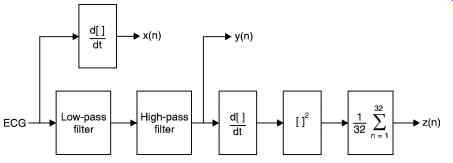
Fig. 30. Filter stages of the QRS detector, z(n) is the time-averaged signal,
y(n) is the band-passed ECG, and x(n) is the differentiated ECG.
Amplitude thresholds are applied to the bandpass-filtered waveform and decision processes make the final determination. Two waveform features are obtained for subsequent arrhythmia analysis-RR interval and QRS duration.
Prev. | Next