AMAZON multi-meters discounts AMAZON oscilloscope discounts
The purpose of this Section is to restate in broad terms the basic premises of electromagnetic theory, and to establish the fundamental concepts and models of electromagnetic phenomena as applied to electromagnetic compatibility (EMC). It’s not intended to give a complete coverage of the topic as this would occupy most of the book. There are many excellent texts on electromagnetics to which the Learner may refer. The topic is also taken up at a level accessible to first-year university students in textbooks like “Introduction to Applied Electromagnetism”.
No secure understanding of EMC may be attained without at least a physical grasp of what electromagnetics is. The analytical equipment normally associated with the subject is also necessary, if basic understanding is to be followed by the ability to make quantitative predictions of EMC performance. This remains so even when numerical predictive simulation packages are used in EMC studies. In the author's opinion, there is no substitute for a core understanding of electromagnetics. It’s therefore proper to devote this Section to this important topic. It’s convenient to examine electromagnetic phenomena under three broadly distinct categories.
First, there are problems where charges are static or they move with constant speed (e.g., direct currents). This type of problem is encountered in DC and low-frequency applications, and the fundamental properties of the field in this limit are that its two aspects, electric and magnetic, can be dealt with separately. Coupling between electric and magnetic field is weak, and it’s possible to develop simple models to examine each separately.
Second, there are problems where charges accelerate slowly, so that although coupling between electric and magnetic fields cannot be ignored, certain simplifying assumptions can be made in interpreting what is taking place.
Finally, in cases where charges accelerate rapidly, no approximations can be made and the most general field models must be employed to account for the strong coupling between electric and magnetic fields.
The first two categories are referred to as the static and quasi-static approximations. The task of this Section is to outline the essential physics applicable in each category, to sketch out the basic models used in making quantitative predictions, and, most importantly, to establish the limits of applicability of each model. In this process the notation, units, and some useful formulae will be given to assist in the more specialized treatment that follows in other Sections.
1. Static Fields
1.1 Electric Field
Static electric charges set up an influence around them, which is described as an electric field. At each point in space, an electric field value is assigned, referred to as the electric field intensity, E, measured in volts per meter (V/m). The amplitude of the electric field does not, however, describe completely the influence of the electric charges. It’s also necessary to assign a direction to the field at each point, much like in a weather map where at each point wind speed and direction are required. In mathematical jargon, the electric field is a vector quantity E described fully when its amplitude and direction are given. The direction of E at each point is that in which a positive electric charge placed there would move. The electric field E(r) a distance r away from a point charge q placed in vacuum (or approximately air) is given by the formula ....
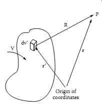
...where if q is in coulombs, r is in meters, and e0 is a constant. The electric permittivity of free-space is e0 = 8.8542 pF/m and then the electric field is obtained in V/m. By the term "point charge" is meant a charge distribution occupying dimensions small compared to r and possessing spherical symmetry so as to look virtually like a charge concentrated at a point a distance r away from the point where the field is observed. The direction of the field is radially outward from a positive charge, as shown in Figure 1.
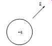
Figure 1 The electric field at a point in the proximity of a spherical
charge distribution.
If the charge distribution does not meet the above criteria, then Eqn. 1 cannot be used directly. Instead the charge is divided into small volume elements dV, each containing a charge ?dV where ? is the charge density. Then, since dV is infinitesimally small, charge ?dV is effectively a point charge and Eqn. 1 applies. The field at any point can then be found by superposition, i.e., by combining the electric field due to each volume element until all the charges have been accounted for. The individual electric field contributions must be combined as vectors to find the total field.
In cases where the surrounding medium is not air but another material, then Eqn. 1 still applies but e0 is replaced by e, the dielectric permittivity of the material used. Materials are normally characterized by their relative dielectric permittivity or dielectric constant er
where e = er e0.
In most, but not all, materials, er is constant and independent of the local value of the electric field or other parameters such as temperature or humidity. The range of er values is remarkably restricted. For most insulating liquids it has a value approximately equal to 3 and in most insulating solids it’s equal to about 5. Notable exceptions are water (er _ 80) and various titanates (er _10,000).
If different materials surround electric charges, the determination of the field is more complicated, as will be explained shortly. It’s also customary to use another quantity to offer an alternative description of the field. This is a vector quantity known as the electric flux density D measured in coulombs per m^2 (C/m^2). In most, but not all, materials, D is parallel to E. The relationship between the two is …
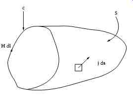
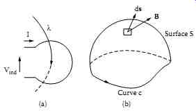
It’s possible to relate, in a compact and elegant way, the electric field (D or E) to its sources (electric charges). This relationship is expressed by Gauss's Law, which states that if, on any closed surface S, the product is formed on the surface area of a small patch ds and the component of the flux density normal to it Dn, and all the contributions are summed to account for the entire closed surface, then the total sum found is equal to the total charge enclosed by S.

[...]