AMAZON multi-meters discounts AMAZON oscilloscope discounts
In trying to interpret the world as it is, humans endeavor to construct models that in some way approximate the behavior of real things. These models are then manipulated by analytical or computational means to predict and interpret the behavior of more complex systems. In electrical work, a very powerful set of models used for this purpose consists of what are described as electrical circuit components. It goes without saying that any model is inherently an approximation to the real thing. A skillful investigator selects the simplest possible model consistent with acceptable accuracy for the type of problem under study. The purpose of this Section is to outline the basic models used in electrical circuit work and describe their advantages and limitations. It would perhaps have been justifiable to start from general models and reduce to more basic ones. Since, however, most Learners are more familiar with the basic models, these are chosen to form the starting point of this treatment. Their relationship to more general models will be established gradually in subsequent sections.
The basic classification of circuit components is divided into lumped and distributed. These are examined in detail in the sections that follow.
1. Lumped Circuit Components
Electrical phenomena require for their description models to represent energy dissipation (losses) and energy supply and storage. From the discussion in Section 2 it’s evident that, in general, two modes of energy storage are required, namely, storage associated with the electric and magnetic fields. In real situations, all energy supply, dissipation, and storage processes are mixed together and distributed over finite parts of space.
The lumped circuit representation is based on the approximation that it’s acceptable to assign each of these processes to individual components, concentrated virtually at a point (lumped) in space. Thus, there is a lumped circuit component with the sole function of representing energy storage in the electric field and so on. These basic circuit components are examined below.
A similar ideal component exists, described as an inductor, to represent energy storage in the magnetic field. The voltage-current relationships across an inductance L are []
The same comments as regards energy exchange apply for inductors as for capacitors. To this list a component representing magnetic coupling between circuits may be added (mutual inductance). Similarly, voltage and current sources are required to represent energy supply. A voltage source is a device that can supply any current, without any change in voltage across its terminals. Clearly, in practice, this can only be approximately correct over a limited range of currents. Hence, a voltage source is an idealization. It may appear that ideal components are of limited use when studying real problems. This, however, is not the case. There are many situations in which these idealizations are good enough in gaining an adequate understanding of real systems. The art of modeling is not to produce the most comprehensive description of a component, but merely to produce one that is good enough for the intended application. The simplicity of ideal components makes them a powerful tool in reasoning about complex problems. More importantly, they may be combined to approximate to a very high degree of accuracy the behavior of real components. This is described in more detail in the next section.
1.2 Real Lumped Components
In many cases, the behavior of real components is difficult to evaluate and quantify accurately. Thus, emphasis will be placed in this section on identifying the circumstances in which real behavior deviates substantially from the ideal. Trends then will be established and quantitative results given whenever possible. Each component is examined separately below.
Resistors - The question posed here is how a resistor deviates from its ideal behavior as a dissipative element. This question may be answered by considering the construction of a resistor. Taking a wire-wound resistor with short leads as an example, it’s straightforward to identify behavior other than that which could be described as dissipation. Since current flows through the leads and the dissipative element, it follows that a magnetic field will be established and, thus, any equivalent circuit of this component must contain an inductance associated with the leads (L_lead) and the resistive element (L_element ), as shown in FIG. 1. Potential differences between different points of such a structure are unavoidable, and hence an electric field will be established around the component.
This in turn implies that a capacitance C must be associated with the resistor R as shown in FIG. 1. All components except R may be regarded as stray components. The way that the stray components have been introduced in FIG. 1 is somewhat arbitrary. Other configurations are possible that can adequately represent the real resistor. At low frequencies, the reactance of the inductive elements is very low; hence, since they are placed in series with R, their contribution is negligible. Similarly, the reactance of the capacitor is high and since it appears in parallel with R, its effects are negligible. Thus, at low frequencies the influence of the stray components is minimal and the component behaves, approximately, as an ideal resistor. At high frequencies, however, the reactance of the stray components dominates the behavior of the real component. Resonant behavior is also possible due to the stray inductance and capacitance. It should also be borne in mind that the values of the stray components are in general frequency dependent.
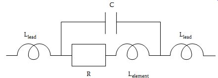
FIG. 1 Equivalent circuit of a real resistor.
Although an exact calculation of these values is a major task, it should be anticipated that, even for a simple piece of wire, capacitances of the order of a picofarad and inductances of the order of a few nano-henry per centimeter length of wire can appear as stray components. Thus, for frequencies exceeding a few megahertz, simple resistors used in circuit construction start to exhibit behavior influenced by stray components. In EMC work, where circuits and components have to meet a demanding specification over a wide frequency range, normally exceeding the normal operating range, the distribution and magnitude of stray components is of paramount interest. It should also be noted that even the value of the resistance R cannot be regarded as constant independent of frequency. It was established in Section 2 that current and magnetic field distribute non-uniformly over the cross section of a conductor. It was found that current concentrates near the surfaces over a thickness of a few skin depths d (Eqn. 3), where .
It follows from this expression that the resistance increases as the square root of the frequency. For conductors with a noncircular cross section, the same principles apply and Eqn. 4 may be used with suitable modifications. Another factor that affects the distribution of current is the proximity of other conductors or components. Any change to the distribution of current in a conductor cross section due to proximity effects will inevitably change the resistance and inductance associated with the conductor.
Capacitors - Capacitors exhibit nonideal behavior for similar reasons as described above. A large value electrolytic capacitor cannot be regarded as being lossless and the capacitor leads contribute their own losses and stray inductance and capacitance, as shown in FIG. 2. This circuit may look unnecessarily complicated, but it brings out the various processes that affect the high-frequency behavior of a capacitor. The lead inductance and resistance are not dissimilar to those associated with a resistive component of similar physical dimensions. Similarly, the stray capacitance Cs is that associated with the electric field established between the capacitor leads. The loss resistance is due to dissipative mechanisms inside the dielectric. If low-loss dielectrics are used, R_loss is very large and can normally be neglected. Its value is related to the loss tangent of the dielectric by the expression

(eqn. 5)
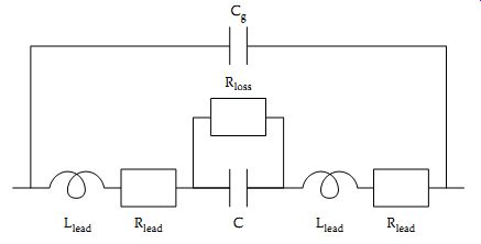
FIG. 2 Equivalent circuit of a real capacitor.
The combined effect of all these factors is to change the character of the impedance presented by a real capacitor. While at low frequencies the impedance decreases with increasing frequency as expected; this situation gradually reverses and, beyond a frequency described as the resonant frequency of the capacitor, the impedance increases with frequency. This indicates inductive rather than capacitive behavior. As expected, the value of the resonant frequency depends, among other factors, on the length of the leads. Common-type capacitors have resonant frequencies of the order of a few megahertz. Lead-through capacitors approach a few tens of mega hertz. Typical behavior for a range of capacitors is shown in FIG. 3, showing how the nature of a nominally capacitive component alters at modest high frequencies. Surface mount capacitors, with much shorter leads, have resonance frequencies that are much higher, but nevertheless the same limitations apply. Some manufacturers of capacitors give an equivalent series inductance (ESL) to account partially for the complex real capacitor behavior at high frequencies.
It’s important to ascertain carefully the high-frequency performance of capacitors used in EMC applications.
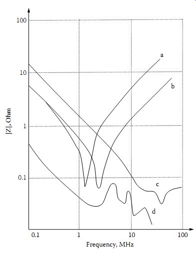
FIG. 3 Magnitude of capacitor impedance versus frequency: (a) 0.25 µF,
10-cm leads; (b) 0.25 µF, 2-cm leads; (c) 0.1 µF, feed-through capacitor;
(d) 4 µF, bushing capacitor.
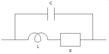
FIG. 4 Equivalent circuit of a real inductor.
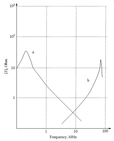
FIG. 5 Magnitude of inductor impedance versus frequency: (a) 10 mH; (b)
6 µH.
Inductors - Inductors are perhaps the most difficult component to design. A possible equivalent circuit is shown in FIG. 4. Resistor R representing losses is usually significant, especially for inductors wound on magnetic cores. It represents several processes, i.e., ohmic losses in the wire and leads, eddy, and hysteresis losses. The latter normally predominate. At low frequencies the impedance increases with frequency.
However, beyond a frequency referred to as the resonant frequency of the inductor, the impedance decreases with increasing frequency. This behavior is characteristic of a capacitor rather than an inductor. Typical behavior for inductors is depicted in FIG. 5. For high-value inductances, the resonant frequency can be quite low (less than 1 MHz).
Inductors of a few microhenry in value have resonant frequencies in the 100 MHz range. The actual value of the inductance depends on the distribution of current. This can be seen even in the simple case of the inductance of a wire. From the discussion leading to the derivation of Eqn. 8 for the internal inductance, it can be seen that it was based on the assumption that the current was distributed uniformly on the wire cross section. This is only one contribution to the total inductance, but it illustrates the range of factors that influence inductance values at different frequencies.
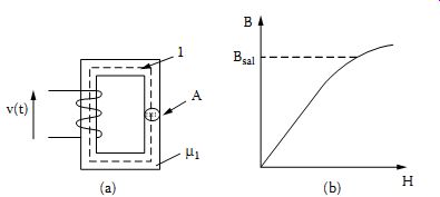
FIG. 6 A nonlinear inductor (a) and the B-H characteristic of the iron
(b).
Another factor that cannot normally be ignored in inductance calculations is the influence of nonlinear effects. In cases where wires are wound on magnetic cores, or are in the proximity of magnetic materials, nonlinear effects may significantly affect inductance values. This may best be illustrated with reference to the simple system shown in FIG. 6. A wire of N turns is wound on an iron former as shown. Actual magnetic cores may be different in shape from that shown. In any case, an effective cross section A and magnetic length 1 may be defined, so that the analysis presented here is of general value in understanding how the inductance of the coil depends on the parameters of the magnetic circuit.
Two fundamental laws may be applied to this circuit to obtain an expression for the coil inductance and a relationship between the applied voltage and the magnetic flux density in the magnetic core. Applying Ampere's Law on a curve coinciding with a mean magnetic line gives:
Assuming that v(t) represents a harmonic voltage of frequency ? and peak value Vpk, the expression above implies that (eqn. 8) From Eqn. 8 it’s clear that the peak flux density in the core depends on the peak applied voltage and its frequency. Magnetic materials have a B-H characteristic of the shape shown in FIG. 6b. If the flux density exceeds the value Bsat , the magnetic field intensity increases disproportionately. This has two implications. First, it means that a much higher current will be drawn by the coil ( Eqn. 6) with undesirable effects on the power supply and circuits feeding the coil. Second, if Bpk >Bsat the magnetic permeability of the iron will decrease substantially. This is clear from FIG. 6b and the relationship µr µ0 = ?B/?H. In turn, the coil inductance decreases substantially. Eqn. 8 offers guidance as to what is likely to happen if the frequency is much lower than that originally intended for the coil. Assuming that the peak voltage remains the same, the magnetic core will operate at a much higher peak magnetic flux density. If this value exceeds Bsat , the coil inductance will be much lower than expected.
It’s therefore necessary to examine carefully the interplay of the various factors mentioned above when a system is evaluated under conditions (such as frequency, peak voltage, pulse duration) that are different to those applicable under normal operating conditions. This is important in many EMC assessments.
The development of realistic models for real components is thus a nontrivial task that must be approached with care. In most cases, simple equivalents can give acceptable semi-quantitative results. Further details may be found in References 1, 2, and 3.
2. Distributed Circuit Components
In real physical systems energy storage and dissipation are mixed together and distributed over relatively large areas. It’s therefore necessary to investigate under what circumstances it’s permissible to separate resistive, capacitive, and inductive behavior and model it by lumped components.
It turns out that in answering this question, the relationship between the physical size of the system and the wavelength of the disturbance to be studied is crucial. Let the size of the system be D and the wavelength of the disturbance be ?. In cases where disturbances of several wavelengths are present, then the shortest wavelength is compared with D. If D << ?, V=N = N AB pk pk pk ?? f then conditions across the network are established practically instantaneously - the propagation time of disturbances is negligible compared to their period. In such cases, it’s a good approximation to lump together various components to model circuit behavior in the most acceptable way.
If, however, D = ?, propagation effects are dominant and a lumped component representation fails to represent accurately a whole class of phenomena observed under these circumstances. It’s still possible to take small sections of the system, of a size that is much smaller than ?, and thus study these sub sections using a lumped parameter representation.
However, when examining the behavior of the entire system, a new way of reasoning is necessary to take full account of propagation effects. The purpose of this section is to develop an understanding of, and techniques for, the solution of distributed networks, i.e., networks for which D = ?.
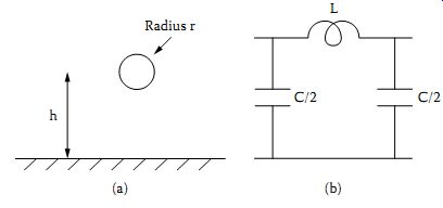
FIG. 7 A wire-above-ground transmission line (a) and its -equivalent
(b).
Let us start first with a few examples to illustrate the circumstances under which a distributed model is necessary. A high-voltage power transmission line of length D = 100 km needs to be modeled ( FIG. 7a).
A typical model used for this purpose is a p-equivalent as shown in FIG. 7b. The inductance L is equal to the inductance per unit length of the line times the line length. The capacitance C is calculated similarly. Under what circumstances is this model an acceptable representation of the line? Consider first the study of power signals (50 or 60 Hz). The wavelength for a 50-Hz signal is ? = 3 × 10^8/50 = 6 × 10^6m. This is much larger than the length of the line and hence the model is quite adequate. Let us now examine whether this model is suitable to study the propagation of lightning-induced transients on this line. These are, typically, unidirectional pulses with a rise-time of 1 µsec. Such a pulse contains a rich spectrum of frequencies, but a substantial amount of energy will be associated with frequencies of the order of 1/tr , where tr is the rise-time of the pulse.
For this example, it’s reasonable to examine whether the model is adequate for the study of frequencies of the order of 1/t _ 1 MHz. The wavelength at this frequency is ? = 3 × 10^8/10^6 = 300 m. This is smaller than the length of the line, hence the model in FIG. 7b is not suitable for studying the propagation of this pulse.
A coaxial cable ( FIG. 8a) 1.5 m in length is used for the transmission of a 100-MHz signal. The cable length can be represented, at low frequencies, by a circuit of the types shown in FIG. 7b. The wavelength at 100 MHz is ? = 2/3 × 3 × 10^8/10^8 = 2 m where the velocity of propagation in the cable was taken to be equal to 2/3 of the speed of light in air.
Since the wavelength is comparable to the cable length, the model shown in FIG. 7b is not suitable for studying this problem.
Finally, let us consider two parallel tracks on a printed circuit board ( FIG. 8b) connecting electronic equipment placed 30 cm apart. Signals with a rise-time of 5 nsec are transmitted along the transmission line formed by these tracks. Treating this problem in the same way as for the lightning pulse and the power line, and taking as the propagation velocity 0.6 times the speed of light in air gives ? = 90 cm. Hence, this line cannot be represented by a circuit of the type shown in FIG. 7b.
These examples illustrate that each physical system may be modeled in different ways depending on the type of problem considered. It’s the task of the investigator to select, in each case, the appropriate model and to obtain solutions. Models of distributed systems and their solutions are presented in subsequent sections. The examples given, and the analyses that follow, refer to transmission lines. There are, however, other distributed circuits that cannot be regarded as transmission lines, and yet their behavior and analysis are very similar. An example is a transformer coil, which at low frequencies may be adequately represented by an inductance or a more complete circuit as shown in FIG. 4. However, when steep fronted pulses are applied to the coil, it behaves very much like a transmission line and may be studied using techniques very similar to those described below.
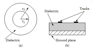
FIG. 8 A coaxial line (a) and a line consisting of two parallel tracks
above a ground plane (b).
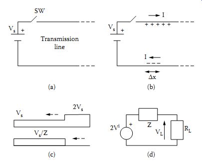
FIG. 9 A parallel-wire transmission line (a), conditions after time ?
? ? fit (b), voltage and current distributions after reflection from the
load end (c), and the Thevenin equivalent circuit at the load (d).
2.1 Time-Domain Analysis of Transmission Lines
Let us consider the parallel-wire transmission line shown schematically in FIG. 9a. The connection of a voltage source on this line will result in the separation and movement of charges and thus in the establishment of electric and magnetic fields. Energy storage in the field may be represented by capacitance and inductance per unit length, Cd and Ld, respectively. These may be calculated if the dimensions and the medium surrounding the line are known ( Section B). The termination of the line at the far end is not specified. The following question is posed:
Immediately after switch SW is closed, what current will flow into the line? More specifically, is this current affected immediately by the actual line termination? The answer to these questions can only be given after a systematic examination of conditions at the start of the line has been made following the closure of the switch. The source will transfer electric charge so that the top wire is left with a surplus of positive charge and the bottom wire with a surplus of negative charge. This situation is depicted in FIG. 9b, where it has been assumed that over a time interval fit this disturbance has progressed into the line a distance fix. The charge induced on each wire is
It’s useful to ascertain exactly what reflections take place when a termination other than an open circuit is present. This can be done easily by replacing the line, as seen from its termination, by its Thevenin equivalent circuit. It’s assumed that a voltage Vi is traveling along the line and is incident on the termination. In the previous discussion Vi = Vs, but the incident voltage would have a different value if the source had a finite impedance, etc. Clearly, the Thevenin equivalent circuit consists of a voltage source equal to the open-circuit voltage of the line 2Vi as shown earlier, in series with an impedance Z equal to the characteristic impedance of the line. This circuit is shown in FIG. 9d connected to the load resistance RL. It’s obvious from FIG. 9d that the load voltage is
As expected, when the load is an open circuit RL ?, the reflection coefficient is equal to one. For a short circuit (RL = 0), it follows from Eqn. 15 that GL = -1. For the special case when RL = Z, the reflection coefficient is equal to zero. This means that the entire line charges to voltage Vi in time t without further reflections. Under these circumstances, the line is described as matched. .
The circuit in FIG. 9d may be generalized to deal with more general terminations. For instance, if the load is a capacitor CL, then RL may be replaced in this circuit by CL and the voltage VL determined in the normal way for a capacitor-charging circuit. Clearly, these analyses are valid as long as no further pulses arrive from further reflections. These more general situations will be dealt with in more detail in Section 8.
Several observations relevant to EMC can be made based on this simple model of propagation and reflection. A line with an open-circuit termination, as shown in FIG. 9a, will carry current pulses of magnitude Vs/Z and duration related to its transit time and the position on the line where the current is measured. For example, the current at the source end will have the waveform shown in FIG. 10a. If losses are neglected then this waveform persists for ever. Otherwise, the current eventually decays to zero. A line with a short-circuit termination does not have a zero voltage across its entire length. The voltage in the middle of such a line is shown in FIG. 10b. If losses are added to this system, the waveform shown decays in an exponential manner. Both these examples indicate the presence of pulses even when the supply is a step voltage. Only in the case of a matched line would a train of pulses be avoided. Clearly, this situation has EMC implications. Further details regarding the propagation of pulses on transmission lines may be found in References 4 and 5.
2.2 Frequency-Domain Analysis of Transmission Lines
In the previous section, the response of a line to a step voltage was examined. Clearly any time-varying input could have been employed instead and the same principles used to obtain a solution. The complexity of such calculations is considerable, however, and they are not normally attempted without computational aids, except for the simplest waveforms.
In many applications, however, the response of a line to a harmonic excitation only is required. In such cases, it’s possible to obtain analytical solutions as shown below.
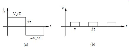
FIG. 10 Current variation at the source end (a) and voltage in the middle
of the line (b).
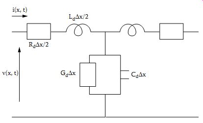
FIG. 11 Electrical model of a line segment.
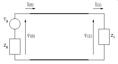
FIG. 12 A model of a complete line in the frequency-domain.
From the EMC point of view, it’s clear that the line termination alone is a poor guide as to the effective impedance seen at the start of a line.
A connection that at low frequencies appears as a short circuit (DC short) looks very different at high frequencies. The material that has been presented in this section is not limited to systems specifically designed as transmission lines. Most wire connections and components behave like distributed components at sufficiently high frequencies, and thus exhibit similar behavior. The importance of these effects may be further illustrated by the following example. A line is formed on a substrate so that the velocity of propagation is u = 0.6 × 3 × 10^8 m/s. It’s required to establish its behavior at a frequency of 300 MHz. The wavelength under these circumstances is ? = 0.6 × 3 × 10^8/3 × 10^8 = 60 cm. Hence a section of this line one-quarter of a wavelength long (15 cm) will exhibit very strongly the behavior described above and due consideration must be given to transmission-line effects. It should be noted that distances of the order of tens of centimeters are typical of track lengths in many electronic systems.
This topic will be examined again in future Sections.
More detailed descriptions of transmission line effects may be found in References 5 and 6.
Prev. | Next