AMAZON multi-meters discounts AMAZON oscilloscope discounts
What is electricity? To begin to answer this question, we have to look at the composition of matter. All matter is made up of atoms, but it is far from simple to describe an individual atom. Atoms are of course far too small to be seen under the most powerful microscope, and we have to infer their construction from the way they behave and from the way they affect various forms of radiation beamed at them. Because nobody quite knows just what an atom really looks like, physicists construct models of atoms to help them explain and predict atomic behavior.
One of the simplest and most straightforward models of the atom was proposed by Niels Bohr, a Danish physicist, in 1913. In Bohr's model of the atom it is assumed that tiny electrons move in orbit around a central, much more massive, nucleus. The electrons are confined to orbits at fixed distances from the nucleus, each orbit corresponding to a specific amount of energy carried by the electrons in it. If an electron gains or loses the right amount of energy, it can jump to the next orbit away from the nucleus, or towards it. A typical atom, drawn according to Bohr's theory, is shown in Figure 1. Electrons towards the outer edge of an atom are held in orbit rather loosely compared with those towards the center.
Electrons in the outermost orbits can easily be detached from the atom, either by collision or by an electric field. Once detached, they are known as free electrons. All materials contain some free electrons.
Materials that are classed as insulators contain only a very few free electrons, while materials that are classed as conductors (notably the metals) contain large numbers of free electrons. These free electrons drift around in the material more or less at random. However, under certain circumstances the electrons can be made to flow in a uniform direction.
When this happens, they become an electric current.
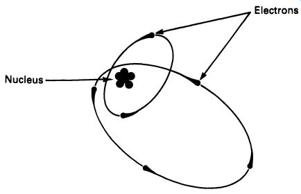
FIG. 1 a model atom, according to Bohr's theory fig 2.2 a single
dry cell
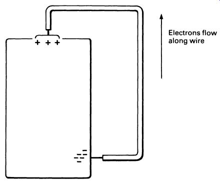
FIG. 3 electrons flowing in a circuit
Let us look at one such example, that of a dry cell. A study of the workings of the cell is not part of a guide on electronics, but details can be found in textbooks on electricity. The illustration in Figure 2 shows a much simplified diagram of a typical dry cell. For our purposes, the important thing is that the internal chemistry of this cell causes the outer casing of the battery to accumulate an excess of free electrons. The center terminal, on the other hand, has almost no free electrons. If the casing and center electrode of the battery are connected by a conducting wire-as shown in Figure 3-electrons will migrate from the casing to the center electrode by flowing down the wire. This current flow is explained by the fact that all electrons carry a single unit of negative electric charge. The electric charge is a form of energy, and may in some ways be regarded as analogous to magnetism. In the same way that similar poles of a magnet repel each other (north repels north, south repels south), so do electrons repel each other. In a normal atom the charges on the electrons are exactly balanced by positive charges on the nucleus. An atom in this state is said to be neutral. Free electrons are repelled by other free electrons, and, as you might expect, are attracted towards areas with a net positive charge.
This is illustrated diagrammatically in Figure 4. Area A has a large number of free electrons, far more than are necessary to balance the positive charges on the nuclei of the atom. Area B has very few free electrons, and indeed a number of the atoms may be missing electrons from their outer orbits and may therefore exhibit a net positive charge. The electrons are repelled by the charge in area A and flow along the wire towards area B. The above is something of a simplification, but illustrates the general principle.
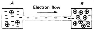
FIG. 4 electrons move from an area having net negative charge to
an area with net positive charge
2.1 UNITS OF ELECTRICITY
It is possible to count (indirectly) the number of electrons flowing along the wire. In order for there to be a useful current, a very large number of electrons must flow. Accordingly, the basic unit of electric current flow is equivalent to around 6.28 x 10¹⁸ electrons per second. This unit of electricity is called the ampere, after Andre Marie Ampere, a French physicist who did important pioneering work on electricity and electromagnetism.
The ampere, often abbreviated to 'amp', is a practical unit of current for most purposes.
In addition to measuring the current flow, we also need to measure another factor, the potential difference between two points. The potential difference between two points is the energy difference between them.
Look at Figure 4 again, and imagine that there is a much larger number of free electrons on side A. This would have the effect of increasing the amount of negative charge on A and increasing the amount of energy available to push the electrons along the wire. Similarly, if side A had only a very few more free electrons than side B, the energy available to push electrons along the wire would be much less. There is a parallel here between the potential difference and water pressure-in fact we can use a 'water analogy' to illustrate the way an electric circuit works. If current flow is the equivalent of a flow of water along a pipe, the potential difference is the amount of pressure available at the end of the pipe. But whereas we might measure pressure in terms of kilograms per square meter, potential difference is measured by a unit called the volt. The volt is named after Alessandro Volta, an Italian physicist who, like Ampere, pioneered work in electricity -he produced the first practical battery. As you might imagine from the water analogy, the current flow is affected by the potential difference. All else being equal, the higher the potential difference-or voltage-the greater will be the current flow.
There is one other factor that would affect the flow of water in the plumbing system: that is the size of the pipe. There is a corresponding factor in the electric circuit, and that is the resistance of the wire. Resistance is a property of all materials that reduces the flow of electricity through them. The higher the resistance, the more difficult it is for current to flow. The three factors affecting current flow are illustrated-with the water analogy-in Figure 5.
The relationship between current, potential difference and resistance was first discovered by Georg Simon Ohm in 1827. It is called Ohm 's Law after him. Ohm's Law states that the current, I , flowing through an element in a circuit is directly proportional to the voltage drop, V, across it. Ohm's Law is usually written in the form: V=IR
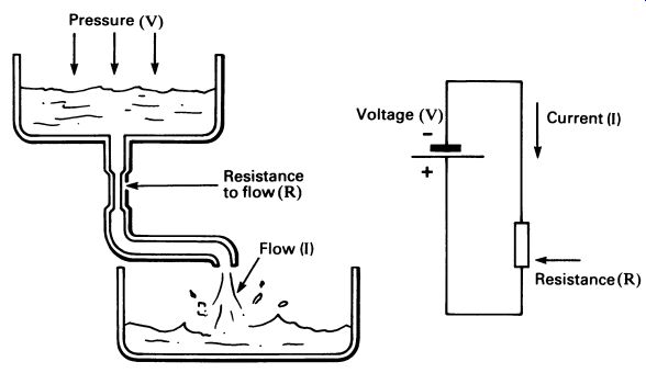
FIG. 5 a plumbing analogy: voltage, current and resistance all have
their equivalents in the water system.
The unit of resistance is called the ohm, for obvious reasons. From the formula above we can see that a potential difference of one volt causes a current of one ampere to flow through a wire having a resistance of one ohm. Given any two of the factors, we can find the other one. The formula can be rearranged as:
v =I R
or
v/R = I
This simple formula is probably used more than any other calculation by electrical and electronics engineers. Given a voltage, it is possible to arrange for a specific current to flow through a wire by including a suitable resistor in the circuit. Similarly, it is possible to determine voltage and resistance, given the other two factors. For some applications in electrical engineering, and for many in electronic engineering, the ampere and volt are rather large units. The ohm, on the other hand, is a rather small unit of resistance.
It is normal for these three units to be used in conjunction with the usual SI prefixes to make multiples and submultiples of the basic units. These are given in the chart in Figure 6. When using Ohm's Law in calculations, it is vital that you remember to work in the right units. You cannot mix volts, ohms and milliamps!
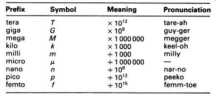
FIG. 6 SI prefixes
2.2 DIRECT AND ALTERNATING CURRENT
So far we have been considering electric current that flows continuously in one direction through a circuit. However, in many applications we will encounter electric current that flows first in one direction and then in the reverse direction. Current that flows first one way and then the other is called alternating current, and a voltage source supplying such a current is called an alternating voltage. Alternating voltages and currents occur in various circuits, particularly in radio and audio, and in power supplies.
Alternating current is used for all mains power supplies because a.c. permits the use of transformers to increase and decrease the voltage, so that the power can be transmitted from place to place using efficient high-voltage transmission lines.
The rate at which the voltage reverses is the frequency of the alternation. One complete cycle, from one direction to the other, and back to the original direction, is the measure: one cycle per second is given a unit, the hertz (symbol Hz) after Heinrich Rudolf Hertz who first produced and detected radio waves. The hertz is equal to one cycle per second, and can be used with the usual SI prefixes; thus 1000 Hz is usually written as 1kHz, etc.
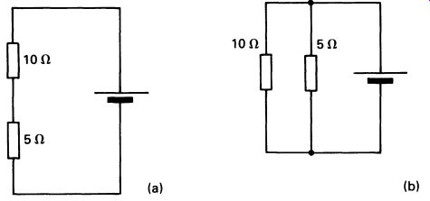
FIG. 7 resistors in series (a) and parallel (b)
2.3 RESISTORS IN SERIES AND PARALLEL
An electrical circuit that draws power from a source of electricity is known as a load. It is possible to connect two loads in an electrical circuit so that all the current flows through both of them. Equally, it is possible to connect them so that current flow is divided between them. The two possibilities are illustrated in Figure 7.
Figure 7a illustrates series connection. In this illustration the loads have a resistance of 10 n and 5 n respectively. To work out the combined resistance of the two loads, for use in calculations involving Ohm's Law, the two values can simply be added together. This is true of any number of resistive loads connected in series-just add the values together, making sure that all the resistances are expressed in the same units (once again, you cannot mix ohms and kilohms). The second case, illustrated in Figure 7b, is less easy to calculate. The formula for working out combined parallel resistance is:
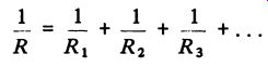
R is the combined resistance, where R1 , R2, etc. are the individual parallel resistances. Working this out numerically for the example in Figure 7b, we get:
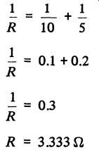
Thus the combined resistance is around 3.3 ohm. It is important at this stage to consider what degree of accuracy is required. My calculator shows that the reciprocal of 0.3 is actually 3.33333333. This seems to be a very high degree of accuracy, but the accuracy is apparent rather than actual. We must consider how accurately the true values of the two resistive loads are known. In order for the calculator's answer to be realistic, we would need to know the resistance of the load to a far greater accuracy than could be measured without the most specialized equipment. We should also consider how accurately we need to know the answer. For most purposes--and bearing in mind the very large number of variables that usually exist within any electric or electronic circuit--it is quite sufficient to say that the combined resistance is equal to approximately 3.3 ohm. In practice, quite complex combinations of series and parallel resistances may be met with. Figure 8 illustrates such an instance. The rule for dealing with part of a circuit like this, and arriving at the combined resistance of all the loads, is to work out any obvious parallel or series combinations first, and progressively simplify the circuit. There is an obvious parallel combination in this figure, so we can work out the combined resistance of the two 100 ohm and two 50 ohm resistors first. Using a calculation like the one above, we arrive at a total resistance of about 16.7 ohm for the parallel combination of the four resistors. Figure 8 has now become more simple-the simplified version is illustrated in Figure 9a.
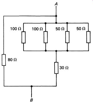
FIG. 8 a complex series-parallel network
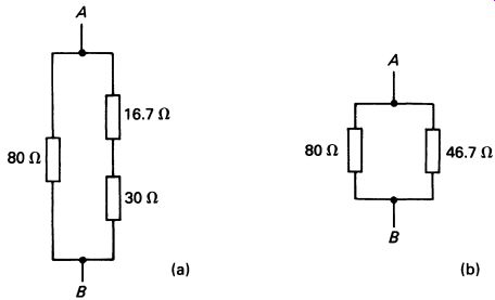
FIG. 9 progressive simplifications of figure 2.8
The series resistors, 16.7 ohm and 30 ohm, can simply be added together to give a total of 46.7 ohm. This leads us to Figure 9b, which is a simple parallel combination which can easily be worked out.
The total resistance between points A and B in Figure 8 is therefore 29.5 ohm---or, in the real world, about 30 ohm.
Change some of the values in the example given in Figure 8 and work through the calculations yourself, to make sure that you are completely happy with these simple calculations. These simple calculations will in fact be a lot simpler if you use a pocket calculator-preferably one that can give you reciprocals. Calculators are inexpensive and any student of electronics should always keep one handy.
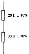
FIG. 10 the effect of tolerance in values
2.4 TOLERANCES AND PREFERRED VALUES
It should be clear that a load having a resistance of, say, 20 ohm is unlikely to have a value of exactly 20 ohm if you measure it accurately enough.
Components having a specified resistance, such as resistors used in electronic circuits, may be marked with a specific value of resistance. But inevitably the components will vary slightly and not all resistors stamped '20 ohm' will necessarily have a resistance of exactly this value. Manufacturing tolerances may be quite wide.
When designing circuits, it is important to bear in mind that components may not be exactly what they seem. As we saw above, this affects the calculations we make, and in any complex circuit we would have to specify circuit values of resistance, voltage and current in terms of a range of values. A resistor marked 20 ohm might, for example, have a resistance of 18 ohm, or 22 ohm. These two limits represent a departure from the marked value of around ± 10 percent. This is in fact a typical manufacturing tolerance for resistors.
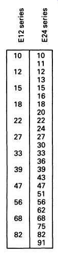
FIG. 11 preferred values of resistors
Preferred values of resistance E12 series is available in all types of resistor E24 series is available in close-tolerance or high-stability only All values are obtainable in multiples or submultiples of 10, e.g. 2.2 ohm, 22 ohm, 220 ohm. 2.2 k ohm, 22 k ohm, 220 k ohm, 2.2 M-ohm, 22 M ohm
Resistance values less than 10 ohm and more than 10 M ohm are uncommon, and may not be available in all types of resistor.
But let us look at the effect of two such resistors connected in a series circuit. Figure 10 shows this. We would expect, using simple addition, that the combined resistance of these two resistors would be 50 ohm. We might base our circuit design on this, and might, for example, predict that this very simple 'circuit' would draw 100 mA from a 5 volt supply. however, let us consider two extremes. If both resistors happen to be at the limits of their tolerance range, then the combined resistance might be 55 ohm. Our circuit would be drawing only 90 mA. If the resistors happened to be at the low end of the tolerance range, then a combined value of 46 ohm could give us a 108 mA current drain from our 5 volt supply. According to the function of the circuit, this might or might not be important.
In some cases we need to be able to specify a resistor more accurately than ± 10 percent. Manufacturers of these components therefore produce different ranges, according to the degree of tolerance permitted. The closer the tolerance, the more expensive the resistor, so it is commercially unwise to specify component accuracy greater than the circuit requires.
Because of the manufacturing tolerance, and because of the impossibility of producing all possible values of resistor, manufacturers restrict themselves to an internationally standardized range of values. Figure 11 lists the available values. Intermediate values are not generally available, but can be made by combining preferred values. It is important to be cautious when doing this, and to bear in mind the tolerance range of the resistors you are using. There is little point, for example, in adding a 3.3 ohm resistor to a 47 n resistor in an attempt to produce something that is exactly 50 n if the tolerance of the combination is likely to be ± 5 ohm. Manufacturers in general restrict themselves to three or four ranges of tolerances. Typically, small resistors would have a tolerance of ± 5 percent, or in some cases± 10 percent. Close-tolerance components of± 21 percent or even ± 1 percent are available, but expensive. Components made to this accuracy would normally be used only in accurate measuring equipment or in particularly critical parts of some circuits.
2.5 CIRCUIT DIAGRAMS
I have already used circuit diagrams, and it is usually fairly clear how circuit diagrams are laid out. You will see many in this guide, and should get a good idea of the way circuit diagrams should be drawn. It is normal to produce diagrams with vertical and horizontal lines, and as few diagonal or angled lines as possible. It is usually convenient to lay the circuit out so that the potential difference in the circuit (or voltage) varies from the top to the bottom of the page: this means arranging the diagram with one power supply line at the top and the other at the bottom in most cases.
Circuit symbols are used to represent different components and different types of components. We have already seen the circuit symbol for a resistor and the circuit symbol for a battery. Other component symbols will be dealt with in context, and explanations will be given where necessary. There are rules about lines in the diagrams crossing, and these must be obeyed rigidly if the diagram is not to be misinterpreted. Figure 12 shows some of the conventions. Figure 12a illustrates wires crossing, but not connecting. Figures 12b and 12c show wires that are connected the little dot is used to indicate a connection.
Sometimes where wires are crossing but not connected the illustrator will use a 'bridge' to emphasize the fact that the wires are not connected.
This is illustrated in Figure 12d; this particular convention is now disappearing. Figure 12e illustrates something which should never appear in circuit diagrams. In all cases where wires are crossing and connected the illustration in Figure 12c should be used. The reason for this is that, if the circuit diagram is printed, the point where the wires cross may 'fill in' in the printing or photocopying process and make it appear that they should be connected when in fact the circuit designer intended that they should not. As you work through this guide you should look at the way the circuit diagrams are laid out, and try to draw neat, clear diagrams yourself. Often, this may mean redrawing--but it is worth the trouble.
In the next section we will be looking at further 'passive' components.
We have already considered resistors, but we shall look at them in more detail-and in the context of the way they are used in circuits. We shall also look at the other two main classes of passive components, capacitors and inductors.
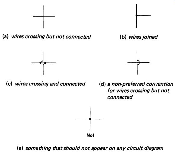
FIG. 12 circuit diagrams --- (a) wires crossing but not connected
(b) wires joined ; (c) wires crossing and connected (d) a non-preferred
convention for wires crossing but not connected ; (e) something that
should not appear on any circuit diagram
QUESTIONS FOR SECTIONS 1 AND 2
1. Describe the difference between linear and digital electronic systems.
2. What is the unit of electric current? What is the unit of electrical potential?
3. Calculate the value of the combined value of the following resistors connected in series: 33k ohm, 18k ohm, 4.7k ohm. If a battery supplies a current of 215 p A through the resistors when they are connected to it, what is the battery's voltage?
4. What is the combined resistance of the following resistors connected in parallel: 220 ohm, 100 ohm, 470 ohm?
5. A 10 k-Ohm and a 5.6 k-Ohm resistor are connected in series. If both resistors have a manufacturing tolerance of ± 10 percent, what, approximately, are the maximum and minimum values of resistance we would expect to measure across the combination?