AMAZON multi-meters discounts AMAZON oscilloscope discounts
53. Definition of an Attenuator
A network that introduces an intentional loss in the transmission of a signal from one point to another, regardless of frequency, is called an attenuator. Generally, a device used for attenuation purposes maintains a fixed impedance at both its input and output ends regardless of the manner in which it is varied.
Attenuators can be designed to have equal or unequal input and output impedances, and to provide varying degrees of attenuation.
They may be balanced or unbalanced, depending upon the requirements of the application. They may be fixed or variable; for example, the T-pad, used to control the level of a remote speaker is a variable attenuator which maintains constant input and output impedance at all frequencies. Fixed attenuators introduce a fixed loss -- as in making a short and long telephone line deliver the same signal to a broadcasting studio - or they may match impedances between a source and load.
Attenuators are designed to work with particular input and output impedances. If worked between sources and loads which differ from the attenuator values, the transmission loss increases. In addition, the design of an attenuator is based on resistive sources and loads, hence an inductive or capacitive load will alter the frequency response.
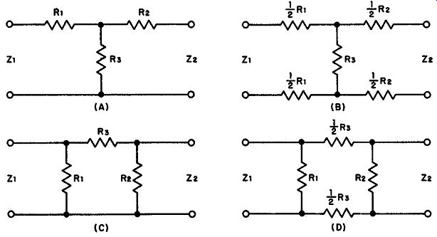
Fig. 56. (A) Unbalanced-T attenuator. (B) Balanced-T attenuator. (C) Unbalanced-,.;
attenuator. (D) Balanced-n attenuator.
54. Fundamentals of Fixed Attenuators
Fixed attenuators normally take the T or ,,,. form and may be unbalanced or balanced (Fig. 56) . In the development that follows, Z1 will always be taken as the larger impedance while Z2 is the smaller. Either may be the input or output impedance of the network.
The loss ratio of an attenuator is normally discussed in terms of power and is defined as: (53)
... in which K is the loss ratio, P1 = power input to attenuator, and P0 = power taken out of network.
In studying the balanced and unbalanced types, note that half the resistance of a given element is transferred to the opposite line to achieve balance.
Assuming that the input and output impedances are not to be equal - such as in an impedance-matching pad -- the ratio of Z1 to Z2 will exceed unity since Z1 is considered the larger of the two impedances. For every ratio of Zl/Z2, there is an associated minimum K that can be realized from the attenuator. This means that in designing an attenuator in which the input and output impedances are fixed by other circuit requirements, a definite minimum loss ratio must be anticipated. This can be determined from the equation:
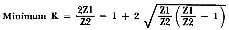
(54)
Equation (54) is solved graphically in Fig. 57 where the minimum possible values of K are plotted as functions of Z1 /Z2. If K does have its minimum value, it can be shown that R2 in either the unbalanced- or balanced-T attenuator must equal zero, and that R2 in either pi network must become an open circuit (i.e., R1 = oo) . 100
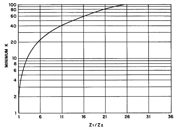
Fig. 57. Minimum K plotted as a function of Z1 /Z2. This graph is useful to
determine the least possible attenuation ratio to be anticipated with fixed
values of input and output impedances.
Example: An attenuator is to be designed that will match a 500-ohm generator at its input to a 200-ohm transmission line. Find the minimum attenuation (or loss ratio) . Solution: The ratio Zl/Z2 = 500/200 = 2.5
From Fig. 57, a Z1/Z2 ratio of 2.5 yields a minimum-K of 7.8. If equation (54) is solved for the same ratio, the result is more exact: 7.87.
Thus, in this situation no attenuator with a loss that is less than 7.87 could be designed.
55. Determination of R1, R2, and R3 in Fixed Attenuators
Let us examine the equations determining the values of the resistors required for fixed attenuators -- (55) through (59) for the balanced- and unbalanced-T, and (60) through (64) for the balanced- and unbalanced-pi network. For the T-type of attenuator we have:
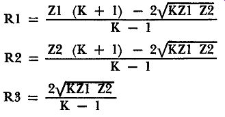
(55)
(56)
(57)
If Z1 = Z2, the foregoing equations may be reduced to the following forms:
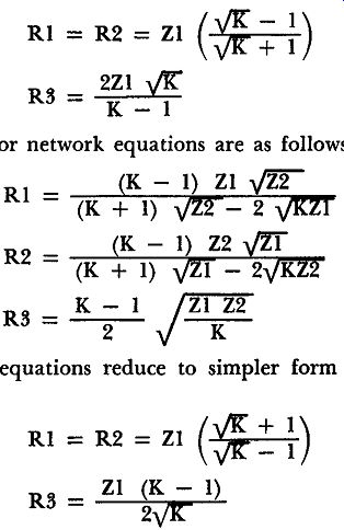
(58)
(59)
(60)
(61)
(62)
The preceding equations reduce to simpler form if Z1 = Z2 as shown below:
(63)
(64)
Example: Using an unbalanced-T network, determine the component values of an attenuator that matches a 500-ohm generator to a 200-ohm load with the minimum possible loss ratio.
Solution: Since the loss ratio is to be a minimum, the value of K must be 7.87 as determined in the previous example for the same input and output impedances. Furthermore, with K = minimum, R2 may be taken as zero, hence this calculation may be omitted. Thus, the determination of RI and R3 are necessary. From equations (55) and (57)
R1 _ 500 (7.87 + 1) - 2-./7.87 X 500 X 200
- 7.87 - 1 R1 = 387 ohms
Fig. 58. The unbalanced-T network is calculated In this example. Note that R1 = zero and Is therefore omitted from the diagram.·
The complete filter thus has the form and values shown in Fig. 58.
Since K is the ratio of power input to power output, the actual network loss in db may be calculated from equation (65)
Loss = 10 log1 • K db
So that in this example the loss is Loss = 10 log10 7.87
= 10 X 0.896
= 8.96 db (65)
Example: A balanced-pi network for the same generator and load as the previous example is to be designed with an actual loss of 20 db. Determine the values of the components required in the network.
Solution: It is necessary to first determine the value of K. Solving equation (65) for K:
Substituting and solving equations (60), (61), and (62)
R3 = 1570 ohms
To form a balanced-pi filter, the value of R3 is divided in half and distributed equally in the upper and lower lines, thus ½ R3 = 785 ohms and the finished attenuator appears in Fig. 59.
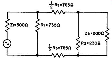
Fig. 59 Balanced-pl attenuator computed.
56. Variable Attenuator Requirements
Variable attenuators are used as volume controls or faders in high quality broadcast equipment, both for transmission and reception.
Their frequency characteristics should be uniform between 20 and 20,000 hz, to prevent the occurrence of frequency distortion. Particularly where such attenuators are used in low-level circuits -- such as the output of microphones or preamplifiers - their noise level must be very low. Unless the noise level is below -150 db, objectionable scratching sounds will be introduced by such low-level attenuators.
Variable attenuators are known as variable pads, constant-impedance gain controls, and faders. Where noise requirements are rigorous, the structure must be protected against dust and stray fields.
For this reason, proper shielding and hermetically-sealed enclosures are necessary.
The last factor we shall introduce is insertion loss. Even when set at minimum attenuation, a variable pad introduces a loss of signal. This loss can be made quite small, especially when Z1/Z2 approaches unity (Fig. 57) ; that is, K approaches 1 when input and output impedances are equal, as in equation (53). For practical purposes, a minimum insertion loss of about 2db is considered standard by most authorities. Although such a loss is generally un important, it may become significant in some applications and should be taken into account.
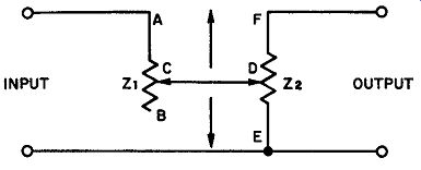
Fig. 60. L-T attenuator for UH as microphone fader or mixer for several micro
phones.
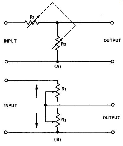
Fig. 62. (A) L-pad attenuator using ganged potentiometers. (B) L-pad redrawn
far the purpose of facilitating analysis.
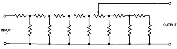
Fig. 61. Ladder attenuator which maintains constant impedance and has only
one moving part.
57. Types of Variable Pads.
L-1 Attenuator: The so-called L-T structure shown in Fig. 60 is frequently used as a microphone fader, and often as a mixer for combining the output of several microphones. If a microphone is connected directly to its load - such as a transformer or the grid of a tube - impedances are assumed to be closely matched. Thus, in designing an L-T fader, it is taken for granted that the input and output impedances are nearly the same so that the insertion loss is generally not more than 2db.
The resistances in the L-T structure are selected so that: (a) the total impedance included between sections AC and DE is equal to the load impedance recommended for the input device. (b) this impedance is maintained regardless of the position of the slider. (c) the impedance contained between F and E matches the load impedance at the output.
Ladder Attenuator: The ladder attenuator (Fig. 61) maintains an essentially constant impedance in both directions through the mid-die of the attenuation range. Although it contains more individual resistors than other types, it has fewer moving parts and is therefore often preferred. The minimum attenuation setting of a ladder fader normally is equal to its insertion loss, generally of the order of 3 to 3.5 db.
Type-L Attenuator: Consisting of two potentiometers with ganged shafts, the L-pad maintains a constant input impedance so that the source always work into the same load. Its operation is more easily understood by referring to the redrawn version shown in Fig. 62B. As R2 is reduced, the load sees a condition which approaches a short-circuit. Simultaneously R1 increases to maintain a constant impedance into which the source works.
Type-T Attenuator: Possibly the most popular of all the unbalanced types of attenuators is the T-pad illustrated in Fig. 63. This arrangement is a modification of the L-attenuator; the modification is introduced to maintain the same impedance for both source and load. The operating principle is, again, easier to understand when Fig. 63 is studied. Consider that all the wipers move up and down together. As R1 increases in resistance, R2 decreases so that the voltage applied between the wiper of R3 and ground becomes smaller. This is the direction of maximum attenuation. The total impedance of the used sections in R1 and R2 remains the same.
Similarly, R3 grows larger as R2 diminishes in resistance, thus keeping the output impedance constant. T-pads are highly favored as microphone faders and also as remote loudspeaker volume controls.
58. fundamentals of Equalizers
Distortionless transmission of signal currents from source, through transmission cable, to the load, requires all component frequencies to be transmitted with equal attenuation or amplification and with equal velocities. Networks containing inductive or capacitive elements do not ordinarily fulfill these specifications. Both attenuation and velocity in such networks are affected by the frequency of the component.
An often used method of correcting frequency distortion in a transmission system is to incorporate an additional network with an attenuation characteristic so related to frequency that the net attenuation of the two will be essentially independent of frequency.
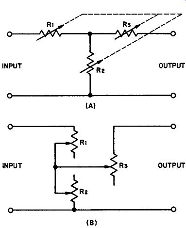
Fig. 63. (A) Conventional drawing of T-pad attenuator. (B) T-pad redrawn to illustrate
the principle of operation.
The same procedure may be used to compensate for delay (or phase) distortion. A combination of transmission and compensation network is used in which the total time of transmission is made independent of component frequency. The wide use of telephone lines in all phases of wired and wireless communication has made equalizer engineering virtually a profession in itself. It is often found that attenuation equalization is sufficient and that delay distortion may be ignored.
Figure 64 illustrates graphically the function of an attenuation equalizer. This is idealized and shows what could be accomplished with a perfect equalizer. In practice, actual equalizers can be made to approach the ideal only over a limited frequency band. The total loss of the combination at all frequencies is greater than the maximum loss of the original system, which explains why equalizers are always associated with amplifiers that can compensate for the loss introduced by equalization.
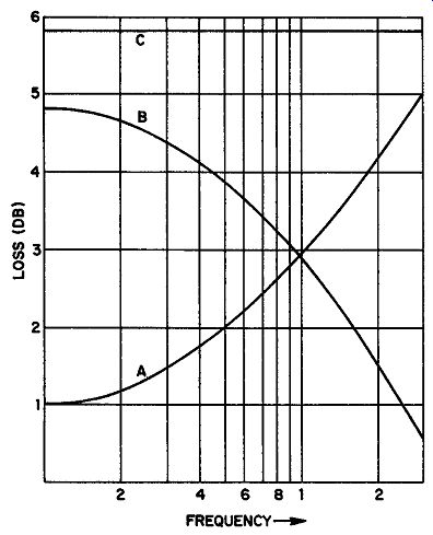
Fig. 64. Ideal equalizer performance. Curve A, shows the attenuation vs frequency
characteristic of the transmission system. Curve B, is the corrective attenuation
applied by the equalizer.
Curve C, represents the resultant curve over the frequency band.
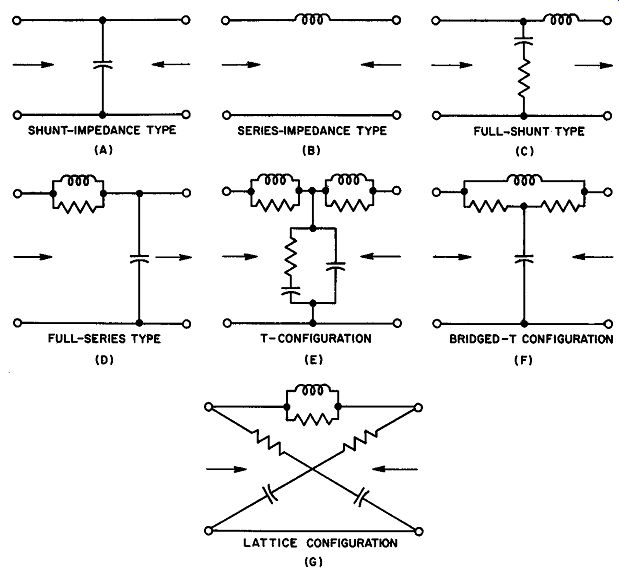
Fig. 65. Equalizer configurations.
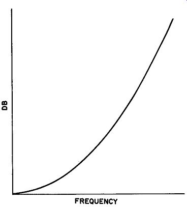
Fig. 66. Any of the seven con figurations shown in Fig. 65 can be designed
to have an insertion loss characteristic similar to this.
59. Equalizer Types
Amplitude equalizer design has been developed to a high order of perfection, largely by the Bell Laboratories and the Research Council of the Academy of Motion Picture Arts and Sciences.1 For the reader who is interested in equalizer mathematics and design, there are excellent papers and articles, as well as special engineering texts, devoted to this subject.
For the purposes of this guide, some mention should be made of the various types of equalizers in use, without attempting to investigate quantitatively the applicable equations.
It is generally assumed that an amplitude equalizer operates from a source impedance that is equal in magnitude to the load impedance. On this basis, it is possible to design several equalizers having different configurations but which offer exactly the same transmission and attenuation characteristics as a function of frequency. Kim ball presents design information for seven of these configurations, each with eight different categories of attenuation characteristics.
The configurations are: 1H. Kimball, Motion Picture Sound Engineering, Princeton, 1938. (An excellent treatment of equalizer engineering design.)
(A) Shunt-impedance type
(B) Series-impedance type
(C) Full-shunt type
(D) Full-series type
(E) T-configuration
(F) Bridged-T configuration
(G) Lattice configuration
Figure 65 presents the general pattern of each configuration for an equalizer that has an insertion loss characteristic (attenuation characteristic) like that shown in Fig. 66. One may well ask why seven different configurations should be described if each duplicates the others in performance. The answer is that one of the seven generally yields component values which are most easily obtained in practical work.
Because of the eight different categories of attenuation characteristics, each of the configurations can be altered to produce any of the curves given in Fig. 67. Above each curve, the series impedance configuration that produces it is shown. Remembering that each configuration can be similarly modified to yield each of these curves, we get 56 possible arrangements. Thus, the equalizer design engineer has a wide field from which to select. It is inconceivable that any practical transmission system could develop frequency distortion characteristics that could not be corrected by one or more of the equalizers illustrated.
60. Phase Equalizers
Phase equalizers are intended to compensate for velocity errors in propagation; that is, a phase equalizer reduces the phase differences between various components of the transmitted signal to a minimum as they arrive at the load. Theoretically, phase equalizers do not affect the amplitude of the signal at all, or do so in a fixed manner, regardless of frequency, so they can be added to existing circuits for phase correction without changing the gain characteristics.
A phase equalizer must be a network in which the phase characteristics can be controlled. Equal transmission times for different frequency components requires that the circuit introduce either no phase shift or an amount of shift that is directly proportional to frequency. This is tantamount to saying that the transmission time must be either zero or constant at all frequencies.
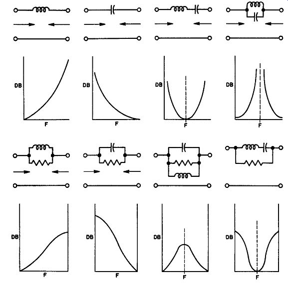
Fig. 67, Possible equalizer insertion loss curves. Although the series impedance
equalizer for each curve is illustrated, any one of the other six configurations
can be designed for the same characteristic.
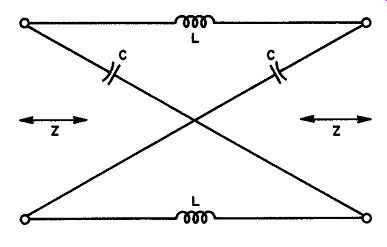
Fig. 68. Lattice-type phase compensation network with zero attenuation characteristic.
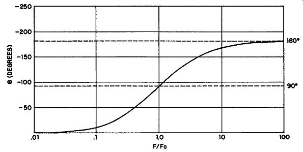
Fig. 69. Phase characteristic of the network shown in Fig. 68. Refer to example
for clarification of Its application.
Although several types of phase equalizer networks are suitable, the most common -- and perhaps the simplest -- is the lattice type shown in Fig. 68. This network has a zero attenuation characteristic and phase characteristics are shown in the curve of Fig. 69. Before we attempt to utilize the curve, we must define the applicable terms and state the pertinent equations.
As a start, let us define certain symbols of importance: f = the frequency at which a certain, known phase shift is desired. As will be shown, f may have several values where the desired phase shift is different for each.
f = the frequency at which the lattice-compensator's phase shift is -90°.
a = the reciprocal of f0 = 1 /f0
z = in the input impedance = the output impedance of the lattice.
theta = phase shift of the lattice in degrees
Using these symbols, the applicable equations for determining L and C of the lattice are: (66)
(67)
Obviously, these equations cannot be used without first deter mining the factor a as defined above. Further, the equations have no meaning unless related to a specific situation in which phase distortion is occurring and requires correction. After the necessary correction is determined, the phase characteristic curve of the lattice is used to determine a. Then the values of L and C may be deter mined from equations (66) and (67) . The technique used is best illustrated by example. The figures have been selected so that the curve will yield exact answers. Usually the engineer is forced to accept approximate information from the curve and correct the values by aligning the actual phase equalizer after it has been installed. When properly handled however, the correction required is small and amounts to slight trimming of the L or C values.
Example: A transmission line, handling frequencies between 10 khz and 20 khz, introduces phase distortion by producing phase shifts at various frequencies as follows: At 10 khz, the phase shift = -27° At 15 khz, the phase shift = -43.5° At 20 khz, the phase shift = -63° As shown in the solution, a phase equalizer is required. Determine the lattice components needed to form a network having a characteristic impedance of 100 ohms.
Solution: (1) First, let us show that a phase equalizer is necessary. If the time delay of a transmission line is linearly proportional to frequency, no phase distortion will occur.
1. In this case, the phase shift at 15 khz would have to be ¾ x -63° if this linear relationship applied since 15 khz is ¾ of 20 khz where the phase shift is -63°. But the actual phase shift at 15 khz is -43.5° rather than ¾ x -63 = -47.25°. Thus, there is a phase error of +3.75°. Similarly, at 10 khz the phase shift should be half that at 20 khz, or ½ (-63) = -31.5° instead of the shift of -27° which actually exists at this frequency. For 10 khz, therefore, the phase error of +4.5°. Obviously, compensation is required to eliminate these errors. To equalize the phase througho1i"t this range, a compensating network having errors the inverse of these must be designed. That is,
Designer Equalizer Error | Frequency
(2)
[1. For a more extended treatment of time delay concepts, see R-F Amplifiers by A. Schure, New York, John F. Rider Publisher, Inc., 1959 ]
Now let us study the characteristics of the curve (Fig. 64) to determine whether there are three values along the f/f0 axis bearing same relationship numerically as 10: 15:20, and which intersect the curve at the correct equalizer error points, as given above. Several trials must be made to approach closest to the desired conditions. In this example, the three suitable points are encircled on the curve. Note
that these occur at f/f0 equal respectively to .4, .6, and .8 and that these numbers are related as 10 is to 15 is to 20. Further, the phase shifts at these values of f/f0 are -43°, -61.5°, and -77°. (3) It must now be shown that the phase shifts produced by the equalizer introduce the right corrective error.
If the phase shift of the equalizer at f/f0 = 0.8 -77°, then for a linear phase characteristic, the phase shift of the equalizer at f/f0 = 0.6 should by ¾ x (-77) = -57.75°.
Actually, the shift is -61.5° and since this differs from -57.75° by -3.75° (see preceding table), the phase error of the equalizer is exactly the figure desired.
Similarly, we analyze the shift at f/f0 = 0.4.
For a linear characteristic, the shift should be ½ (-77) = -38.5°. Its actual phase shift, however, is -43°. The equalizer error is then -43° - (-38.5°) = -4.5°.
This phase error also corresponds with the desired value given in the table. We now have all the factors required to calculate the necessary values of L and C for the lattice equalizer.
(4) The value of f0 is next determined. Since this is the frequency at which the phase shift of the equalizer is -90°, and since f/fo = 0.8 at f = 20 khz, then f0 must be 25 khz. This follows from the fact that f/f0 at a phase shift of 906 is unity, hence:
0.8 20 khz l
= fo and thus f0 = 25 khz.
(5) The value of L may now be determined from the definition of a and equation (66) given on page 81. Since a = l/f0 , then a = 1;25000 = 4.0 X 10^-5. Substituting in equation (66) : 4 X 10-• X 102 L = 6.28 (Note: the impedance characteristic of this equalizer was specified as 100 ohms. Hence, the factor 102 in the numerator) . L = 0.64 millihenries (6) C is determined from equation (67)
0.64 X 10-• C = 10' C = 0.064 X 10-• farad
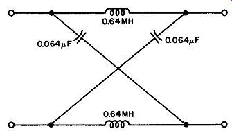
Fig. 70. The lattice phase equalizer computed for the example. Note that this
network is symmetrical and therefore may be used In either direction.
C = 0.064 microfarad.
The complete lattice, with values is given in Fig. 70.
61. QUIZ
1. Describe the function of an attenuator. Specifically, what function is served by a fixed attenuator in contrast to a variable type.
2. What is meant by the loss ratio of an attenuator?
3. How can one determine the minimum possible loss ratio of a fixed attenuator?
4. Derive equation (58) from the equations that precede it.
5. What is the loss ratio (K) of an attenuator having equal input and output impedances of, say, 500 ohms?
6. What is the minimum loss ratio of an attenuator that matches a 200-ohm transmission line to a 400-ohm load? Find the actual loss in db of this attenuator.
7. Describe four types of variable attenuators and describe the characteristics of each.
8. What is an equalizer? What kinds of equalizers are there?
9. How does an amplitude equalizer differ from a phase equalizer?
10. What essential characteristics must a phase equalizer possess to be effective?