AMAZON multi-meters discounts AMAZON oscilloscope discounts
37. Filter Classifications
Wave filters, sometimes known as Zobel filters, are generally described as constant-k or m-derived filters and represent a unique family. Many of the filters described in previous sections are basic ally either constant-k or m-derived types and may he analyzed with techniques used for generalized wave filters. Design procedures for wave filters are based upon complex mathematics and will not he dealt with in this section. The technician can derive substantial benefit from a discussion of filter types and filter structures, using the minimum mathematics needed for comprehension, and bypassing study of the derivations of the equations and charts needed for design work.
[“Theory and Design of Electric Wave Filters", Otto Zobel, Bell Tech J, vol. II, p.1., Jan. 1923]
The same is true of bridged-T and parallel-T networks. We shall study the general principles of their functioning rather than the development of design techniques. For those interested in de sign of any type wave filter, this section is recommended as a preliminary step, followed by a thorough study of design procedures that can he found in any of the numerous modern electrical engineering texts.
Constant-k and m-derived filters may be placed in roughly four classifications: Low-pass filter: This has a pass (or transmission) band theoretic ally starting from zero frequency to the frequency at which cutoff is desired, and an attenuation band from the cutoff frequency to infinity.
High-pass filter: The reverse characteristics obtain attenuation band from zero to the cutoff frequency and a passband from cutoff to infinity.
Bandpass filter: Two cutoff frequencies are specified, high and low. Transmission will occur between these frequencies and attenuation on either side of them.
Band-elimination filter: Again, two cutoff frequencies with attenuation between them and transmission on either side of the cutoff frequencies.
Bridged-T and parallel-T networks will be discussed later, as they are of specialized design.
38. Effectiveness of Attenuation and Transmission
In the attenuation-band of a given filter, the characteristic impedance of the filter is a pure reactance. If the load that terminates the filter is equal to the characteristic impedance of the filter, the generator at the input will see a pure reactance. For this condition, no power is transmitted to the load, hence, attenuation is perfect. This ideal situation is modified in practice because filters are often terminated in pure resistances and an impedance mis match exists between the filter and load. This is reflected back so that the input impedance of the filter becomes slightly resistive.
Thus, some power will be transmitted by the filter into the load even in the attenuation band.
In the transmission band of the same filter, however, the characteristic impedance is a pure resistance and, if the load is equal to the filter's characteristic impedance, the input generator will be working into a pure resistance. Since an ideal filter contains only reactive or non-dissipative elements, in the theoretical situation all of the generator power is transmitted to the resistive load. In actual practice, of course, the filter components contain resistance so that some power dissipation occurs here as well as in the load. Hence, a practical filter transmits most, but not all, of the generator power to the load in its transmission band.
39. Characteristic Impedance
If a filter is terminated by a load having an impedance such that the filter is caused to have the same input impedance, the filter is said to be terminated by its characteristic impedance. Sometimes known as surge impedance, the characteristic impedance of a filter may be found from: (31)
where …
Z0 = characteristic impedance of the filter
Za = input impedance with output terminals open-circuited
Zb = input impedance with output terminals short-circuited.
The term surge impedance is often used with reference to trans mission lines and has a similar significance. If a transmission line is terminated by a load equal to the surge impedance of the line, all the energy will be transferred to the load and there will be no re flections of energy back along the line. It is helpful to view filter sections as portions of an infinite line drawn to show its various impedance elements as lumped components. We will use this approach in the forthcoming paragraphs.
40. Basic Filter Configurations
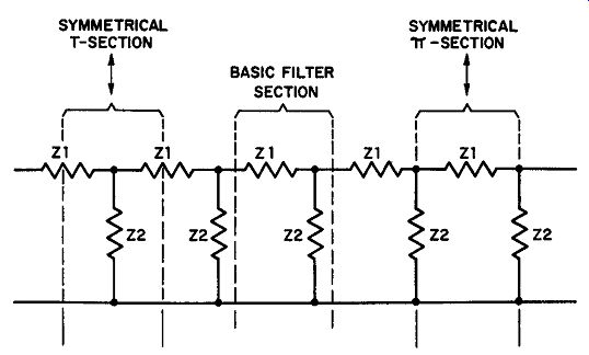
Fig. 43. Symbolic representation of a long transmission line, showing its
distributed impedances as lumped elements of recurring nature.
Transmission lines are recurrent structures having continuously distributed impedances. Two wires in space have, besides their ohmic resistance, shunt capacitance and series inductance along the line. Signifying any type of impedance with the resistor symbol, a long line may be drawn as shown in Fig. 43. Each series element is labeled Z1 and each shunt element Z2. The basis of filter design is a full L section consisting of series element Z1 and shunt element Z2, shown between the labeled broken lines in Fig. 43.
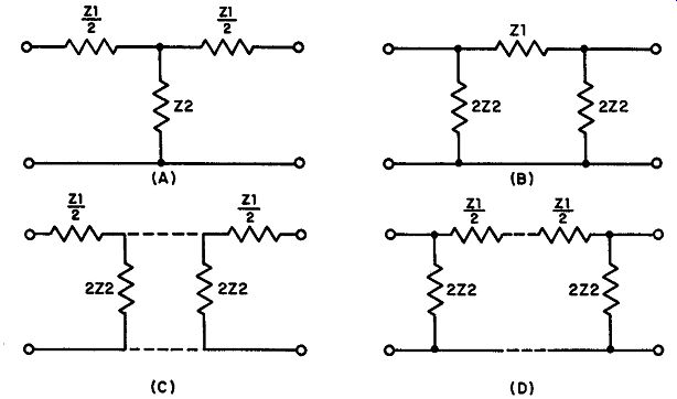
Fig. 44. (A) Symmetrical T-section type of filter configuration, mid-series
terminated. (B) Symmetrical it-section configuration, mid-shunt terminated.
(C) Symmetrical T-section divided into two half-sections by replacing Z2 with
two impedances in parallel, each being evaluated as 2Z2. (D) Symmetrical it-section
similarly divided, each Z1 being replaced by Zf/2.
A wave filter normally makes use of small, symmetrical sections because the number of sections is finite rather than infinite, like the line. One section, called the symmetrical T-section, is obtained by dividing each of two adjacent series elements in half and including between them one shunt element. Thus, the value of each series element (or half-element) is now designated as Z1/2 while the shunt element remains Z2. (Fig. 44A). Because the symmetrical T section is cut from the infinite line by bisecting each of two series elements, it is known as mid-series terminated.
The symmetrical ;re-section configuration is obtained by cutting down the centers of two successive shunt elements of the infinite line, including one series element between them (Fig. 44B) . Since a shunt impedance thus bisected has a resulting impedance of twice the initial value, the filter configuration shows an evaluation of 222 for each shunt element and ZJ for the series element. Such a section is said to be mid-shunt terminated.
For design and analysis purposes, either type of configuration may be divided into half-sections as shown in Fig. 44 (C) and (D).
41. Characteristic Impedances of Filter Sections
The characteristic impedances of symmetrical T and :n:-sections are given by the following equations:
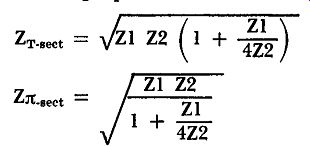
(32)
(33)
Examination of these equations shows that the characteristic impedances of the two networks depend upon frequency. It is difficult to terminate either one with a simple network.
As a special case, if a filter is terminated in a pure resistance R which is made equal to __/Z1 Z2, it may be shown that equations (32) and (33) may be written:
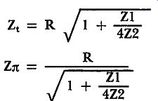
(34)
(35)
The significance of the expression __/Z1 Z2 will become more evident in the next section.
42. Constant-k Filters Defined The simplest and most common type of filter section is that in which the shunt and series impedances are intentionally selected so that:
__/Z1 Z2= constant = k (36)
for all frequencies. Furthermore, the terminating resistance for the filter is chosen to be equal to k, that is R = k so that the equations (34) and (35) are applicable. In constant-k filters, each inductance in the shunt and series arms is associated with a capacitor in the series and shunt arms, respectively. In an ideal filter the shunt and series arms are made of non-dissipative elements wherever possible. Assigning the No. I to series elements and the No. 2 to shunt elements, as before, the required relation between the elements for a constant-k filter (that is, to maintain the product of 21 and 22 constant) is: (37)

Constant-k filters may be set up in any one of the four major classifications (high-pass, low-pass, bandpass, and band-elimination) . In the paragraphs that follow, we shall examine the transmission characteristics of each of these classifications, with applicable equations.
Remember in each case that equation (37) is adhered to exactly, so that the product of Z1 and Z2 is always a constant and is always equal to the terminating impedance of the filter.
43. Low-Pass Constant-k Filter
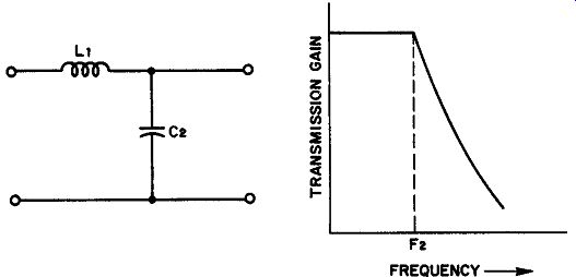
Fig. 45. Schematic diagram and transmission curve of a low-pass constant k
filter. Note that the elements are non-dissipative.
A low-pass constant-k filter contains an inductive series element (L1) and a capacitive shunt element (C2). Its transmission curve is given in Fig. 45 with its schematic diagram. This is an idealized drawing in which the filter elements are non-dissipative and there are no reflection losses at the terminals. In a practical filter, where there is some power dissipation in the elements and where impedances are not perfectly matched, the cutoff is somewhat more gradual than the curve indicates.
The values of the elements are found from equations (38) and (39).
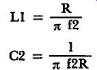
(38)
(39)
... where f2 = frequency where attenuation begins. The reader should test the constant-k quality of these values by setting up the ratio as given in equation (37) to show that the square root of L2 over C1 comes out equal to R.
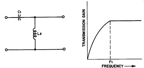
Fig. 46. Schematic diagram and transmission curve of a high-pass constant-k
filter.
44. High-Pass Constant-k Filter
As illustrated in Fig. 46, a high-pass constant-k filter contains a capacitive series element and an inductive shunt element. In this case, the frequency at which full transmission begins is denoted by fl. The same idealization assumptions are made for the high-pass filter as for the preceding filter and for others that follow, unless otherwise noted. Element values may be determined from equations (40) and (41).
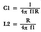
(41)
45. Bandpass Constant-k Filter
The bandpass constant-k filter (Fig. 47) is considerably more complex than the high- or low-pass types. Containing an inductive and capacitive element in the shunt and series legs, four equations are required to determine the constants. Frequencies fl and f2 are the lower and upper limits respectively of the transmission band.
The design equations are given in (42) through (45). It is again suggested that the reader test these equations against the ratios given in equation (37) to ascertain for himself that the constant-k relationship between elements is maintained, regardless of the filter's complexity.
(42)
(43)
(44)
(45)
46. Band-Elimination Constant-k Filter
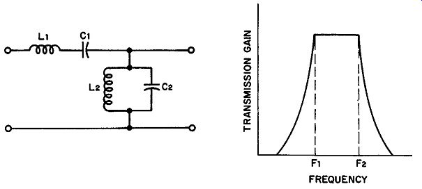
Fig. 47. Bandpass filter of the constant-k type, showing an idealized transmission
curve.
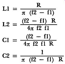
In the band-elimination constant-k filter, the series leg contains an inductance and capacitance in parallel while the shunt leg contains these elements in series. Figure 48 presents the schematic dia gram and transmission characteristics of this filter. The applicable equations are given in (46) through (49).
(46)
(47)
(48)
(49)
Fig. 48. Band-elimination filter of the constant-k type showing Idealized trans mission curve.
47. m-Derived Filters Defined
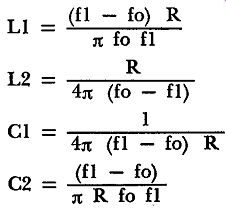
Even the idealized transmission curves of the constant-k filters demonstrate a gradual cutoff characteristic that is unsatisfactory for many applications. Sharper cutoff may be realized by incorporating additional impedances in the shunt or series arms so that infinite attenuation occurs at some frequency beyond cutoff. With the constant-k type of filter used as a prototype, for example, the addition of another impedance in one of the arms can produce the kind of modified response shown in Fig. 49. In this case a T-section low-pass filter (A) is altered by adding L2, a shunting impedance, in series with C2B. This filter has a very high attenuation (low impedance) at the frequency where L2/C2 resonates; ideally, the L2/C2 combination can shunt a zero impedance across the line, causing infinite attenuation. When the two components are properly selected, this frequency of infinite attenuation (f oo) can be placed anywhere in the attenuation band.
Since the filter in Fig. 49B, is derived from the constant-k proto type as we shall show in the next section, the impedances are related by a constant ( called m) , the network in (B) is known as an m derived filter.
48. m-Derived T-Sections
It would be desirable to be able to join different filter sections of the general type shown in Fig. 49 with each section having an infinite attenuation frequency at a different point in the attenuating band. In this manner, a high value of attenuation could be realized and maintained through the entire region.
Fig. 49. Modification of constant-k filter response by adding additional shunt
Impedance.
To do this without undesirable reflections, one must be certain that the characteristic impedances of the different sections are equal to each other at all frequencies. If the characteristic impedances could be matched at all frequencies - the various filter sections would also have the same transmission band. This would have to be true because in only the transmission band is Zo a pure resistance.
Consider first the constant-k filter of Fig 50A.
The characteristic impedance of this filter section is given by equation (32)
(32)
Now let us derive another filter section having new branches called Z1' and Z2' with a characteristic impedance of Zo'. Furthermore, let us say that Z1 and Z1' are related by a constant multiplier m as in equation (50) .
Z1' = mZ1 (50)
If the characteristic impedances of both filters are to be the same, then we must find a configuration such that
Zo = Zo' (51)
1. Equation appears earlier under this number
Fig. 50. (A) Constant-k prototype filter from which the m-derived filter in B is obtained. (B) m-derived filter having the same characteristic impedance as the constant-k prototype.
To fulfill equation (51), it should then be possible to set the characteristic impedances of the two filters in Fig. 50 equal to each other as follows:
Squaring both sides and simplifying, we have:
Now substituting mZ1 for each Z1' in accordance with the assumption made in equation (50) , the equation above may be written as:
Solving this equation for Z2' yields
The Z1 factor may be cancelled so that:
… and the terms combined to give:
… more simply written as:
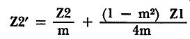
(52)
Equation (52) , therefore, implies that if the impedance Z2' in Fig. 50B is given the configuration specified by the right members of the equation, the characteristic impedance of the constant-k filter in (A) will be identical with the characteristic impedance of the derived filter in (B) . The development above also demands that the series arms be given the value of mZ1 as provided in equation (50). Thus, the series arms contain one component each (mZ1). The shunt arm must contain two components, one with an impedance of Z2/m and the other with an impedance of (1-m^2) Z1/4m.
Since the filter has been derived from a constant-k type in which each series arm is Z1/2 (Fig. 50A), then each series arm in the de rived filter is mZ1/2. Thus, the complete filter appears as shown in Fig. 51.
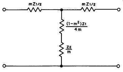
Fig. 51. m-derived filter containing proper impedance values as compared with
constant-k prototype so that its characteristic impedance equals that of the
prototype.
By using equations (50) and (52) and varying the value of m, any number of sections can be designed, differing in respects but having the same characteristic impedance. Such filters can be linked without reflections between them to obtain virtually any attenuation characteristic desired. The question arises as to the order of value that m may assume. The upper portion of the shunt impedance having the value:
(1 - m^2) Z1 4m provides the answer to this question. In order that this value maintain the proper relationship at all frequencies, the numerator must not be permitted to become negative. Hence, m may vary only between zero and +1.
49. Examples of m-Derived Filter Sections
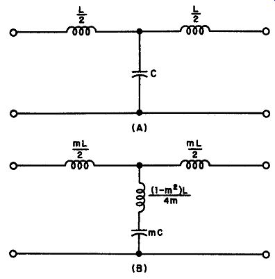
Fig. 52. (A) Symmetrical T section mid-series terminated low-pan filter (constant-k).
(B) m-derived low-pan filter obtained by applying equations (50) and (52) to
the prototype .
To illustrate the design of simple m-derived filter sections from constant-k prototypes, we might examine a common low-pass and high-pass filter configuration. For example, the constant-k prototype of a symmetrical T-section, mid-series terminated (see Fig. 44A) arranged for low-pass characteristics appears in Fig. 52A.
In the m-derived filter of Fig. 52B, note that the capacitive element is mC (rather than C/m) because of the inverse relationship between impedance and capacitance. Since L and Z are related directly, the inductive component values have the same form as in equation (50) and (52) . A symmetrical T-section high-pass filter, first in its prototype form, then in its m-derived form, is illustrated in Fig. 55. Note the application of equations (50) and (52) to the derivation of the values of the series and shunt arms.
Constant-k prototypes may also be used to construct m-derived pi-sections. The same general procedure obtains the relevant equations. Repeat: it is not our purpose to discuss design details, but you may follow through with specific filter forms based on general principles and examples in this section.
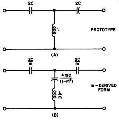
Fig. 53. Symmetrical-T high pens filters of the constant-k prototype and the
m-derived forms.
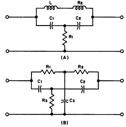
Fig. 54. (A) Bridged-T network consisting of LCR components. (B) Parallel-T
network containing R-C components, only.
Bandpass and band-elimination filter configurations in both constant-k and m-derived forms can also be designed, using similar mathematical approaches. Design formulae and equation derivations may be found in any of the excellent electronic handbooks now available in the public libraries.
50. Bridged-T and Parallel-T Configurations
Figure 54 illustrates two other types of filter networks of specialized design. In general, these systems are used as band-elimination filters, feedback networks for frequency-selective amplifiers and oscillators, and calibrated bridges for measuring devices. They are characterized by their ability to produce high attenuation for a single frequency or group of adjacent frequencies over as narrow a band as desired. They are also capable of producing large phase shifts -- either lagging or leading as the design dictates. With the proper selection of components, the maximum phase shift can be as much as 180°. It is also comparatively easy to build bridged-T and parallel-T networks with a negative transfer function (i.e., output voltage 180° out-of-phase with the input voltage). Such a net work can be applied to the construction of a single-stage vacuum tube oscillator having exceptional frequency stability) . The bridged-T network in Fig. 54A is unique in that there is no theoretical limit to the minimum width of the attenuation band it can introduce. Actually, the practical limitation is set by the Q of the inductor in the bridging leg. Because of its sharp, narrow attenuation properties, the bridged-T network is often applied where a truly null feedback loop is needed. To illustrate, we shall briefly consider the general structure of a frequency-selective amplifier.
51. Frequency-Selective Amplifier
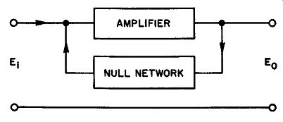
Fig. 55. General plan of a frequency-selective amplifier, using a null network
in the feedback loop.
If a negative feedback amplifier is set up with a null network in the feedback loop (Fig. 55) , an amplifier having sharp frequency selective characteristics can be designed. The amount of feedback at the null frequency theoretically is zero, so that the gain of the amplifier at the null frequency is the same as its gain without feedback. On either side of the null frequency, the attenuation of the filter drops sharply, causing a greater effective negative feedback and consequently far less amplifier gain.
Bandpass-selective amplifiers, having a flat passband rather than a single peak, as is obtained with resonant circuits, can be designed by using several independent feedback stages, staggered in frequency.
The frequency to which each feedback stage is tuned may be deter mined as are staggered tuned circuits.
52. QUIZ
1. Give the four basic filter classifications. What are the distinguishing characteristic (s) of each group?
2. If the input impedance of a filter network is 400 ohms with its input terminals open-circuited, and 4 ohms when the input terminals are short circuited, what is the surge impedance of the network?
3. Explain what is meant by a mid-series terminated filter section. How does a mid-shunt terminated section differ?
4. Why do equations 32 and 33 show that the characteristic impedance of a network is a function of frequency?
5. Prove that equations 34 and 35 may be derived from equations 32 and 33.
What assumption is made in this derivation?
6. Define a constant-k filter section. Why is this type of filter desired more than similar sections not having constant-k characteristics?
7. Using equations 38 and 39, determine the values of L and C necessary to form a low-pass filter in which the attenuation begins at 1500 hz. The characteristic impedance of the filter is to be 600 ohms.
8. How does the physical structure of a constant-k bandpass filter differ from a constant-k band-elimination filter?
9. Describe in your own words how an m-derived filter differs from a constant-k type. What are the principal advantages of the m-derived network as contrasted with the constant-k?
10. Draw a bridged-T and parallel-T configuration. State how the applications of these filters differ from those of the constant-k and m-derived networks.