Rack-mount digital audio processor using predictive delta modulation with compansion (CPDM). Output: conventional TV signal (North American standards) which can be recorded on any high-quality VCR. Power consumption: 60W. Dynamic range: 110dB (maximum 1kHz signal to A-weighted noise 20Hz-20kHz), 105dB (unweighted). Frequency response (sinewave 100mV input): 20Hz-20kHz ±0.5dB. THD (1V input, 1kHz): less than 0.05%. Wow & flutter: less than 0.01% (unweighted), less than 0.006% (weighted RMS). Anti-aliasing filtration: -3dB at 37kHz. Sampling/bit rate: 644kHz. Maximum input/output levels: 24dBm. Mike preamp (optional): adds less than 1dB of noise for mikes between 100 and 1k impedance. Inputs: line 5k, differential; edit audio 20k, differential; mike 100k, 6.8k if phantom-powered (48V); video & sync 75 ohms. Outputs: line 47 ohms, single-ended, drives 600 ohms, switchable to balanced; edit audio 100 ohms, single-ended; headphones 150 ohms. Dimensions: 19” W by 3” H by 11.5” D. Source: long-term manufacturer’s loan. Price: $4600 plus $375 for mike preamplifiers. Manufacturer: dbx Inc., 71 Chapel St., Newton, MA 02195. Tel: (617) 964-3210.
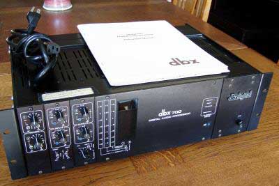
ABOVE: dbx 700 PCM processor
As ALF would say, “There’s more than one way to cook a cat.” We’ve been so overwhelmed with linear pulse-code modulation (PCM) recording, we forget there are other ways to pass from the analog domain to the digital.
One of these is delta modulation. The Greek delta (which in its upper-case, block-letter form, looks like an equilateral triangle) is the mathematical symbol for the difference between two quantities; accordingly, in delta modulation, we record not the absolute value of a signal sample, but the c4fference between successive samples.
Delta modulation isn’t new. It’s been used for years as a simple way to reduce the necessary bandwidth required to transmit TV signals. Poke your nose up against the CRT, and you’ll see that one horizontal line is very much like the preceding or succeeding line. The lines’ content doesn’t change rapidly, so we don’t need much information to describe the difference between one line and the next. If we transmit just the difference information, there’s a big reduction in the required band width. (Major changes, which require a lot of transmitted information, are uncommon and don’t significantly drive up the bandwidth requirements.)
The same principle can be applied to ordinary PCM. The difference between two samples can never be as large as the absolute maximum level of the program material— sounds do not jump 96dB in 1/50,000th of a second!—so our 16 bits, which would normally cover the full dynamic range of the signal, can be applied to the much narrower range of sample differences. If we designed a system on the assumption that the difference between one sample and the next was never more than 1% of peak signal level (a conservative estimate), we’d gain a 100-fold improvement in resolution! (Not bad.) Or, we could use fewer bits, for resolution comparable to that from conventional PCM. An additional advantage, besides the gain in resolution (or a reduction in bandwidth), is that we no longer have to worry about the signal’s absolute level. When we “run out of numbers” in conventional PCM, the signal is clipped to produce a nasty-sounding error. But with a delta-modulation PCM system, the analogous situation produces slew-rate limiting—the recorded difference between samples is not as great as the actual difference—a less offensive distortion.
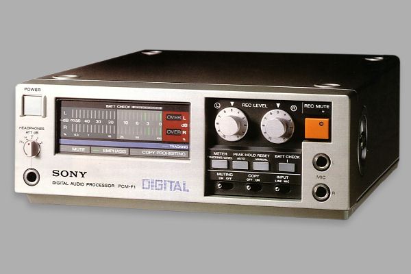
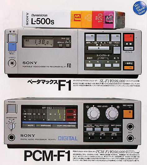
ABOVE: the dbx 700's main compitetion (ca. late 1987) -- the Sony PCM-F1
The problem with such a system, though, is that it requires some pretty hairy hardware. Not only do we have to sample the signal as accurately as in regular PCM, but we have to compute a very accurate difference between successive samples. PCM hardware is complex enough as it is. Why should we have to go to all this trouble for a slight improvement?
There’s a way out of this dilemma. Suppose we could make a systematic guess as to what the next sample value would be. By systematic, I mean that the guess is not random. It follows a strict set of rules, so the same set of initial conditions always results in the same guess. Both the encoder and decoder would obey these rules. Therefore, we would only need to transmit the difference between the predicted value of the signal and its actual value. The decoder can figure out the predicted value on its own, then apply the difference signal for correction.
Such a system is called (surprise!) predictive delta modulation. PDM creates an estimated model of the signal in much the same way a painter does a quick sketch on the canvas before he fills in the details, then transmits a code that describes whether the estimate is larger or smaller than the actual value of the next sample. If the sampling is fast enough (greater than about 500kHz), there usually won’t be too big a difference between one sample and the next. The difference between the sample and the estimate will then be so small that we can accurately describe it with a code of just one bit!
The basic PDM circuit (from the dbx manual) is shown in fig.1. It looks complicated, but it’s really very simple. There are three sections which I’ll explain one at a time.
Let’s start by saying “Hello!” to our old friend, the capacitor. We can charge a capacitor by applying a voltage to it. The capacitor’s charge (in coulombs’) is found by multiplying the applied voltage (in volts) by the capacitance (in farads). Or:
Q = CV
(I know you’ve seen that before!)
It works just as well the other way ‘round. If we stuff Q amount of charge onto a capacitor, the capacitor’s voltage will increase by
V=Q/C
Note that the change in voltage is determined only by the capacitance and the change in charge. A given amount of charge added (or subtracted) will increase (or decrease) the capacitor’s voltage by exactly the same amount, regardless of the total amount of charge on the capacitor. Got that? Good.
Now look at the right-hand section of the schematic. (We’ve separated it so you won’t be confused by the rest of the circuit.) The triangle represents a high-gain amplifier. A capacitor is connected from the output to the input. This configuration is called an integrator, because it adds up (integrates) the charge pumped into (or pulled out of) its input.
The exact way the integrator performs its magic is too complicated to go into. (I’d need to explain operational amplifier circuits, an article in itself.) But here’s the important part. The injected charge is transferred to the capacitor, and the amplifier’s output is the same as the capacitor voltage (given by Q/C). For example, if the capacitor were 2uF, and we pumped in 0.5uC, the output voltage would rise by 0.5/2.0, or 0.25 volts. Likewise, if we pulled out 0.luC, the voltage would fall by 0.1 / 2, or 0.05 volts. The integrator is, of course, adding up all these little deposits and withdrawals. Therefore, the instantaneous output of the integrator is simply the running, net charge, divided by the value of the capacitor. Simple, nest ce pas?
Where does the charge come from? From those two little circles marked pos and neg. They’re charge pumps. One pushes charge, the other pulls. Like the two sides of Alice’s mush room, one makes the total capacitor charge grow larger, the other makes it grow smaller. When either is activated, it inserts (or removes) a precisely defined quantity of charge.
As you should have figured out by now, it’s the integrator voltage that models the input signal. By pumping in or pulling out charge, the encoder tries to make the integrator voltage match the input. If the integrator voltage is less than the input, charge is pumped in. If the integrator voltage is greater than the input, charge is removed. But how does the encoder know whether to add or subtract charge?
Easy. It uses a comparator. (That’s the triangle on the left.) A comparator is simply a high-gain differential amplifier. That is, it subtracts one input from the other, and amplifies the difference.
Assume the differential amp has a gain of 1 sagan (one billion times). If the difference between its two inputs is 1 billionth of a volt, the output will be 1 volt. Of course, a billionth of a volt is awfully small. (The circuit’s random noise is much larger!) 10 microvolts is a more likely difference, buy times 1 sagan is 10,000 volts. How do we get 10,000 volts out of an amp that runs on an 18 volt power supply?

FIG. 1. BASIC SINGLE-INTEGRATED DELTA MODULATOR
We don’t. An amplifier’s output is limited to the power supply voltage. The amp simply tries its darndest to meet the 10,000V requirement. The result in engineering jargon is that the amp slams up against the rails.” That is, the output jumps up to the power-supply voltage (or down to ground), because that’s the highest (lowest) it can go. Which way it jumps depends on the polarity of the difference between the inputs. If it’s positive, the amplifier moves to the positive rail, and vice-versa. It’s highly unlikely that the integrator’s output will ever be close enough to the input to produce a bounded output (i.e., one that sits stably between the rails). There fore, the comparator will constantly jump back and forth, high and low, depending on the relative polarity of the signal input and the comparator output.
Of course, we still haven’t explained just how this twitching voltage selects Ipos or Ineg. That’s done by the little thingy in the middle. It’s called a flip-flop. As you might guess from the name, it’s a circuit whose output can take one of two states—high or low. High and low can be any two voltages we like; the important thing is that the flip-flop’s output must be one of these two voltages.
There are several types of flip-flops. The one shown here is a D-type (“D” stands for “data”). The flip-flop has a special data input: when the flip-flop is triggered, its output jumps to the same logic level (high or low) as the data input. The trigger signal is simply a steady frequency (in the model 700, it’s 644kHz). Each time the trigger goes positive (once per cycle), our D flip-flop is triggered, and the data at the input is transferred to the output. The data, in this case, is the comparator output. Therefore, every time the flip-flop is triggered, its output switches to match the current output state of the comparator.
The little dotted line in the schematic is supposed to suggest that this logic level selects between Ipos and Ineg. Indeed, that’s just what happens. The comparator “decides” whether the integrator’s output is higher or lower than the signal input. The flip-flop is set to this logic state, which in turn deter mines whether we will inject or remove charge. And so on, as long as there’s an input. (By the way, it’s this train of logic highs and lows that constitutes our digitization of the input.) That’s it! See how simple it is?
I can already hear objections from The Peanut Gallery. “If all you ever transmit is the difference between the actual and estimated signal values, how can you ever reach the absolute level of the signal? Isn’t that what you want to recover?”
Good question. Yes, it’s the absolute value we want. Imagine this not-unlikely situation. There’s no input. Then—suddenly!—a really big sinewave drops by. The comparator notices that there’s like, wow, a really gross difference between the integrator and input voltages. So it doles out one of its little dribs of charge, and 1/644,000th of a second later, compares again. Whoops! It’s still behind, so it dumps in some more charge, and so on. Will it ever catch up?
Technically, no. What happens is that the input signal falls behind. The sinewave eventually reaches its peak level, then falls. At some point on its decline, the input voltage drops below the integrator output. At this point, the integrator voltage and the input aren’t too different. Everything settles down, with the estimated value close to the absolute value.
The decoding process is identical to the coding. We simply use the logic highs and lows to switch the Ipos/Ineg charge pumps. The integrator output is then a kind of zigzag approximation of the original input. Of course, the zigs and zags are at 644kHz, so it’s easy to filter them out. We’re then left with (we hope!) the original waveform. Of course, the actual circuit is rather more complex. A different type of integrator, which produces less quantization noise, is used. The noise level still isn’t low enough for critical use, so compression (similar to the system used in MTS) is placed ahead of the encoder. There is even digital compression; if the encoder produces more than nine “highs” in a row, the compressor is told to squash the signal even further. Of course, all the compression is undone in playback.
But the nicest feature of a companded delta modulation system is its noncritical level set ting. The encoder has to be severely over- driven before it goes into slew-rate limiting, and be badly under-driven before noise be comes objectionable. You don’t know what a relief it is not to have to worry about clipping the encoder when recording a live performance. (I did it a few times with the Nakamichi DMP-100, but the clipping was so brief as not to be readily audible.)
Of course, every advantage has its tradeoff. The nature of delta modulation imposes a limit on the maximum slew rate that can be handled. For a given signal amplitude, doubling the frequency doubles the slew rate. So although delta modulation can accommodate very high frequencies, the maximum input level varies inversely with the frequency. dbx gets around this problem by weighting the record-level display correspondingly, to pre vent over-recording.
Physical features
The 700 is a professional product. Though light enough to take into the field, it’s intended to sit in an equipment rack; its basic con figuration, therefore, is a unity-gain, line- in/line-out device. All input and output sockets are XLRs. As shipped, the line outputs are unbalanced. They can be converted quickly to balanced operation with a pair of (sup plied) resistors.
The front panel is imposing at first, but the layout is completely logical: each function has its own module, and they proceed from left to right, in input-to-output order. A few minutes’ perusal of the instruction book will make you an expert.
Mike preamps are an option, and plug into the first slot on the left. Once installed, a toggle switch selects between line and mike. (There is no mike/line mixing.) A second switch selects 48V phantom microphone powering. A stepped rotary control sets mike gain from 20 to 60dB, in’ 10dB steps.
The record input module is next. A switch at the bottom chooses between record and playback—unlike the Sony PCM units, the 700 cannot simultaneously encode and decode. The 700 has a pair of conventional analog outputs that can feed the video recorder’s audio tracks (either linear or Hi-Fi). In playback, these supply quick, easy cueing, since there’s no need to wait for the decoder to lock in. A second switch determines whether these analog outputs will be straight or compressed. (Oddly, this compression is not dbx, and there is no playback expansion.) The record inputs are unity gain. However, there are two options. You can move a toggle switch to ADJ, and turn a knob to vary the gain over a + 10 to -60dB range. If only a small change is needed, you switch to TRIM, and use a screwdriver to turn a trimpot. Its range is ± 10dB.
The input module has CLIP lights preceding and following the gain stage. dbx claims that a single cycle at 10kHz is enough to light them, if the level is too high. Keep an eye peeled, and lower the gain (at the appropriate point) if either comes on.
The next module, naturally, is for playback. It, too, is unity-gain, and it has the same ADJ and TRIM options as the recording module. There is, however, only one CLIP light, at the input. At the bottom of the module is a head phone jack (with gain control) that’s live during both record and playback. A toggle switch selects DIGITAL or EDIT, which switches the headphones from the decoder output to the analog cue tracks during playback.
The last “module” is actually a cover plate for several cards underneath. All the audio and video displays are here. The audio-level display is an LED bar graph with three modes, chosen by a toggle switch. The mode is indicated by red, yellow, and green LEDs.
RECORD LEVEL (weighted) is just that. The scale is from +20 to -40dB; 0dB does not correspond to unity gain. The weighting takes into account both the pre-emphasis of the compander and the limitations of the delta-modulation encoder.
CALIBRATION has a 15dB range (from + 5 to -15dB), unweighted, in 0.5dB steps. 0dB is line level. This mode is for setting levels and balances.
SIGNAL LEVEL runs from +20 to -100dB, in 4dB steps, unweighted. It’s used during playback to examine the dynamic range of the music or the noise floor of the equipment feeding the 700.
On the other side of this panel are the three LED5 that comprise the video display. The red VIDEO UNLOCK indicates that there is no video input, the yellow STANDBY shows that there is a video signal but the decoder hasn’t yet locked in, and the green VIDEO LOCK comes on when the delta demodulator is fully functioning.
Below these three lights is a red ERROR CORRECT LED. Unlike the PCM-F1, the 700 has the common decency to let you know when it’s fixing things. And, unlike PCM units, there is no interpolation. Either the bad bit is properly corrected, or it’s missed altogether. As explained, an occasional uncorrected error wreaks no havoc.
This light is a great way to check for tape dropouts. (With Sony ES-HG, there’s an error correction about every two seconds; with Maxell HGX, they occur about every 30 seconds!) In any case, the circuitry reconstructs the signal and feeds it to an error-corrected output on the back panel, for dubs.
Fortunately, the 700 doesn’t look like a Christmas tree. Only three lights are normally on: power, display mode, and either the record light or one of the playback status lights. Any other light indicates an exceptional condition—48V powering, nonstandard gain, error correction, or clipping. A nearsighted person can stand 20 feet away and still know just what the 700’s doing.
My first 700 was DOA; it recorded, but emitted only a low buzz during playback. dbx said it was a show unit that hadn’t been checked, and replaced it. The second unit (reviewed here) recorded and played properly, but had a flaw in the display circuits. The left display showed a continuous “ghost” signal. Since 80% of everything I’ve reviewed in the last six months was defective, broke down, had some design flaw, or featured a combination of these problems, I wasn’t fazed by this. I did, however, have a minor problem with the input sockets (both mike and line). My XLR plugs had to be pushed in very hard before they would lock in place, and the left-channel plugs wouldn’t lock at all. (There was no problem with the outputs.) This appears to be due to some subtle (!?) incompatibility between XLR brands. I wedged in the plugs, then dressed the cables so they wouldn’t be knocked loose. I had no problems after that.
The instruction book was up to dbx’s usual superb quality: friendly and informal without silliness; clear and simple without inaccuracies. It was a pleasure to read, something I can’t say about most manuals. The ability to write literate manuals is common among New England hi-fi companies. It’s hardly surprising, considering the area’s literary tradition.
Stereophile, August 1987
Sound quality:
The sound quality was checked in the best possible way—by using the 700 to make live recordings. On one outing, I brought another VCR and the Nakamichi DMP-100 (flee Sony PCM-F1) for comparison. I made up a cable so the mikes could feed both digital processors simultaneously. (I didn’t use an external mike preamp. I wanted to see how each processor sounded with its own preamp, since this worst-case situation is the way most of our readers would use these products.)
Before going any further, I want to dissociate myself from the opinions about the PCM Fl and DMP-100 expressed in Stereophile’s “Recommended Components” listing in Vol.10 No.3. Although I switched from analog recording to the DMP-100 because of its superior sound quality, I’ve never claimed, publicly or privately, that it was “99.7% perfect.” It ain’t. Comparing tapes of the same performance, it was immediately obvious that the Nakamichi DMP-100 and the dbx 700 did not sound alike. The most striking difference was in instrumental timbre. On the DMP-100, almost everything was lighter and brighter in texture, even bass percussion instruments! This was especially noticeable on violin, which sounded as if it were all strings and no wood. Nor did the 700 fully capture the “body” sound of the violin, but it came a lot closer. There was a more solid sense of the fundamental, and less exaggeration of the overtones.
Another difference showed up on brass. The DMP-100 was noticeably grundgy. The 700 had a deliciously smooth brass tone that in no way lacked “flatulant blattiness” or attack.
Of course, “different” is not “better.” Was the DMP-100 adding something, or the 700 taking something away? I checked this by comparing the direct output of the 700 with the same signal sent through the DMP-100. (The latter has simultaneous encode/decode.) The DMP-100 made the 700 recording sound like the DMP-100 recording, lightening and brightening the instrumental texture. The proper conclusion, then, is that the dbx 700 is the more accurate of the two processors.
The obvious question arises: are these sonic differences due to fundamental differences between PCM and PDM? Unfortunately, there’s no way to tell. They could just as well arise from differences in the analog circuits that surround the digital processors. The only way to know for sure would be to swap the analog sections, an impractical task.
To sum up:
To say that I am delighted with the dbx 700 is an understatement. It’s more accurate than the DMP-100 (and, by implication, the PCM F1). Although bulkier, it’s not especially heavy, and the power supply is built-in. (The DMP-100/PCM-F1 needs an outboard unit.) Best of all, I don’t have to chew my nails worrying whether or not I’m going to clip the processor during loud passages. On sound quality alone, it goes right into Class A, with the Nakamichi and Sony dropping into Class B.
I also like the 700’s open architecture. In principle, any module can be modified or upgraded, something not really practical with other digital processors. (If you’ve dismantled a PCM-Fl, you’ve seen its tightly wadded innards.) Think you can design a better sounding line module? Go to it! Further, since delta modulation uses off-the-shelf components, the 700 will probably be repairable well into the next century
Of course, $4975 is a bit pricey for a digital processor, even for our well-heeled readers (Price is not a consideration for entry into Class A.) Still, it’s a fine-sounding unit, and any serious amateur or professional recordist should give it a careful listen. Highly recommended.
== == FOOTNOTES == ==
1. A coulomb is an Avogadro’s number’s-worth of electrons, about 6E23. It’s named after Melvin Coulomb, the French music-hall comic who discovered how easy it was to build up an enormous static charge by shuffling across the carpet. Mel died tragically, the victim of a jealous husband whose wife’s derriere he (Mel) had zapped once too often. In accordance with French legal precedent, the husband was acquitted.
2. We assume there’s no output transformer to step it up.
3. Simple math. Doubling the frequency doubles the number of waveform transitions in a given time. To make twice as many transitions, we have to move (slew) twice as fast. Right?
4. As I write this, dbx tells me that they are selling the 70C out of stock” They will make at least one more production run of the 700, but I would suggest that if you want a 700, now is the time to buy.
== ==
ALSO SEE:
== == ==