Waveform Distortion Analysis [Scope Waveform Analysis (1963)]

Waveforms contain information which requires more or less interpretation. This requirement has been touched on in previous Sections. Distortion is encountered in a vast number of forms, and each type of distortion has a cause. If you recognize the reason for a particular type of distortion, you can proceed with confidence to correct the defect that is indicated.

REACTANCE VERSUS FREQUENCY

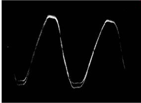
Fig. 7-1. Scope waveform with vertical input lead open-circuited.

One of the simplest types of distorted waveform reproduction is observed when the vertical input leads to a scope are open circuited. The floating input lead picks up 60-cycle hum voltage from stray fields. The 60-cycle "sine-wave" display is also distorted (Fig. 7-1) , due to exaggeration of harmonics (attenuation of low frequencies) with respect to the source waveform in the 60-cycle line.

An open test lead is capacitively coupled to the power wiring in the wall and at the bench. This capacitance is small; hence, stray-field sources are high-impedance sources. Since a scope has high input impedance, it can display the voltage from a high-impedance source. Because the source is capacitively coupled to the open test lead, the coupling is reactive and its ohmic value decreases with increasing frequency. A 60-cycle stray field is basically a 60-cycle sine wave, but it almost always contains harmonics-principally odd harmonics due to the small nonlinearity of transformer cores. Thus, the 60-cycle stray field contains frequencies of 180 cycles, 300 cycles, and so on. The higher harmonics are coupled more strongly to the open test lead and are emphasized in the stray-field pattern. This is the reason that the waveform in Fig. 7-1 departs significantly from a sinusoidal shape and appears flattened on the peaks.

The "fuzz" in the waveform is due to antenna action of the open test lead, which picked up the carrier of a local AM broadcast station. The "fuzz" is broader at the bottom of the waveform than at the top because the service-type scope exhibited amplitude nonlinearity.

Part of the distortion in the Fig. 7-1 waveform originated in the scope. Two other types of distortion which may be produced by a scope are shown in Fig. 7-2. When a 60-cycle waveform is intensity-modulated at a 60-cycle rate, one-half of each cycle has a high intensity, while the other half has a low intensity. This intensity modulation results from incomplete filtering of the high-voltage power supply. Another common type of distortion produced by a scope is horizontal compression due to nonlinear sawtooth deflection. An experienced operator learns to distinguish between distortion arising in the scope itself and distortion caused by defects in the circuit under test.

STRAY-FIELD PICKUP CONSIDERATIONS

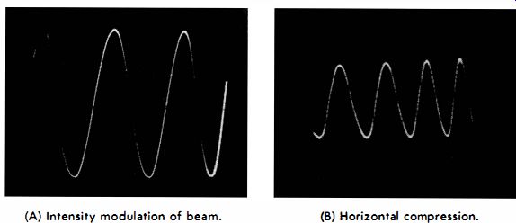
Fig. 7-2. Two types of waveform distortion. (A) Intensity modulation of beam. (B) Horizontal compression.

Beginners sometimes complain about stray-field pickup as if it were a design defect in a scope. Any instrument with high input impedance responds to stray fields. Thus, a VTVM responds to stray fields when it is set on its low-voltage ranges and the input cable is open-circuited. Waveform distortion due to stray-field pickup is avoided by using a shielded input cable to the scope. Open test leads are suitable only for testing in low-impedance circuits. If a scope has exposed vertical input terminals, you may note stray-field distortion even when a shielded input cable is used, particularly if you bring your hand near the vertical input terminal while adjusting the scope controls.

For this reason it is preferable to use a coaxial connector instead of exposed binding posts for the vertical input terminals.

WAVEFORM DISTORTION DUE TO NON-UNIFORM TUBE CHARACTERISTICS

Vertical compression ( Fig. 7-3) sometimes occurs in the scope, but it is more often due to a defect in the circuit under test. An audio amplifier, for example, always starts to exhibit vertical compression when driven near the limit of its dynamic range. The reason is seen from the chart of plate characteristics in Fig. 7-3. When the grid is driven strongly negative, the characteristics become more closely spaced; this results in diminishing output. Again, when the grid is driven positive, the grid input impedance becomes very low, and the source may not be able to supply the grid-current demand. Therefore, the drive voltage falls, and the output diminishes. It is evident that negative peaks, positive peaks, or both may be compressed or clipped, depending on the operating conditions of the tube and the amount of drive voltage applied.

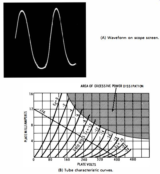
Fig. 7-3. Distortion due to nonlinear amplifier-tube operation. (A) Waveform on scope screen. (B) Tube characteristic curves.

The area of excessive plate dissipation is shown in Fig. 7-3.

Since the load line is below the "forbidden area," it might be supposed that the tube could not be damaged by overdrive. It is true that overdrive cannot cause rated plate dissipation of the tube to be exceeded. However, when the grid is driven positive, it starts to dissipate power and may become red hot. Grid dissipation must be considered in addition to plate dissipation, and if positive grid drive is substantial, the tube can be damaged.

Distortion vs. Operating Point

It can be seen from Fig. 7-3 that the grid bias might be chosen to place the operating point anywhere along the load line. Thus, the operating point might be placed at -4 volts or at -18 volts.

A common method of setting the operating point is to use a cathode resistor of the proper value for the desired operating point. For the tube depicted in Fig. 7-3, a bias of about -10 volts will permit the maximum dynamic range with minimum distortion.

If the bias is set at -4 volts, it is evident that the tube will go into grid-current distortion first as the drive voltage is increased. On the other hand, if the bias is set at -18 volts, the tube will go into cutoff distortion first as the drive voltage is increased. When a tube must be operated over a large dynamic range, it is necessary to choose a midrange bias point which will cause the tube to enter grid-current distortion and cutoff distortion simultaneously at high values of drive. This might not necessarily be the operating point for minimum harmonic distortion at moderate drive.

When grid-current distortion occurs, it first appears as compression of the positive peak in the grid voltage. As the grid-current distortion increases, compression changes to clipping-this may be a horizontal clipping or a diagonal clipping (Fig. 7-4) . Whether the clipping is horizontal or diagonal depends on the grid-coupling circuit time constant, component values, and the frequency of the drive signal. Remember when checking waveforms in an amplifier stage that the waveform is reversed in polarity from grid to plate. Note that when cutoff distortion occurs, waveform clipping is horizontal-the plate simply stops conducting and no further voltage change occurs until the drive signal passes through its peak excursion.

This is not to say you might not observe apparent diagonal clipping due to cut-off distortion, especially when checking low-frequency operation. Some scopes will distort a 60-cycle square wave, for example, and the clipped peak of a 60-cycle sine wave is processed in the scope like a 60-cycle square wave.

This is another situation in which distortion arising in the scope might be incorrectly charged to the amplifier under test.

A DC scope avoids this possibility of confusion in low-frequency tests; however, it is seldom possible to use a DC scope directly at the plate of a tube, because the plate-supply voltage throws the beam off the screen. Instead, a large blocking capacitor must be used in series with the vertical lead to the DC scope. A value of 0.5 mfd or even larger may be required to completely eliminate tilt in low-frequency tests.

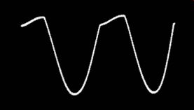
Fig. 7-4. Waveform produced by severe clipping in grid circuit.

EVALUATING SMALL AMOUNTS OF DISTORTION

You cannot observe 5% distortion in a sine wave, and even 10% harmonic distortion may be evident only to the eye of a trained operator. Hence, a linear time base is not very useful for evaluation of small amounts of distortion; a cyclogram evaluation is preferred. A cyclogram is obtained as shown in Fig. 7-5A. A small amount of amplitude distortion is present in Fig. 7-5B, as evidenced by the slight departure of the trace from a straight line. Here again, it is necessary to distinguish between distortion originating in the amplifier under test and distortion that might occur in the scope itself. In case of doubt, remove the amplifier from the test setup and check the scope directly for amplitude linearity.

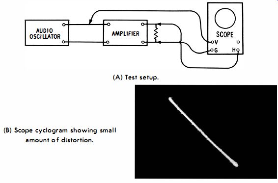
Fig. 7-5. Method of checking amplifier for distortion. (A) Test setup. (B) Scope cyclogram showing small amount of distortion.

Amplitude linearity Check

To check a scope directly for amplitude linearity simply connect the "hot" output lead from an audio oscillator to both the vertical and horizontal input terminals of the scope. Connect the ground terminal of the scope to the ground terminal of the audio oscillator. A perfectly straight diagonal line should appear on the scope screen-if it does, the scope amplifiers are linear. On the other hand, if a curved line is displayed, the scope amplifiers are nonlinear. While it is possible to make allowances for scope nonlinearity in analyzing waveforms, this is difficult at best; it is preferable to use a scope which has good amplitude linearity.

In case the scope itself is not entirely linear, note the departure from linearity in the cyclogram when the scope is tested directly. Then, when you proceed to test an audio amplifier, observe whether the same departure from linearity is displayed -- if so, the amplifier under test is linear. On the other hand, if the pattern is different from the reference pattern, the amplifier is nonlinear. Amplifier nonlinearity could improve the reference pattern in particular circumstances-the essential point is that any departure from the reference pattern indicates amplifier nonlinearity.

TRANSIENT DISTORTION

Transient distortion may originate in the circuit under test or in the scope itself. Fig. 7-6 illustrates severe ringing of a chroma waveform. In most cases this type of distortion results from an excessively high and sharp peak in the IF- or video amplifier response. However, it can also result from the use of a scope preamplifier which has a steeply rising high-frequency response. A preamplifier with this characteristic is sometimes employed to compensate for falling high-frequency response in a scope. Thus, if a scope has flat response out to only 1 or 2 mhz, an attempt is sometimes made to obtain an over-all characteristic that is flat through 3.58 mhz by utilizing a preamp with a steeply rising high-frequency response.

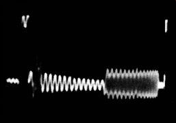
Fig. 7-6. Severe ringing in chroma waveform display.

When the required compensation is not extreme, this expedient is satisfactory. On the other hand, when the required compensation is quite substantial, transient distortion is produced. The amount of high-frequency rise which can be tolerated depends on the rise time of the signals to be processed. If a signal has a comparatively slow rise, transient distortion will not appear; if the signal has a fast rise time, transient distortion develops in any amplifier which has a rising high-frequency response. Square-wave generators, for example, usually have a much faster rise time than color-bar generators.

Distortion Due to Phase Shift

Even if each stage in a scope vertical amplifier has a flat frequency response, the amplifier will ring on steep wavefronts if the frequency response drops off suddenly instead of gradually. For example, a scope might have each stage adjusted for flat frequency response to 4 mhz, after which the response takes a sudden "nose dive." This sharp cutoff characteristic will cause the scope to produce transient distortion of square waves with fast rise times. The reason for this difficulty is that the phase characteristic of an amplifier becomes highly nonlinear through a sharp cutoff region. A nonlinear phase characteristic will cause the higher harmonics in a square wave to ring, much as an upward-sloping frequency response will do.

To obtain a reasonably linear phase characteristic through the cut-off region of an amplifier, it is necessary to make the frequency response taper off gradually. This taper is controlled by the peaking-coil circuitry in the amplifier. Series peaking alone develops a gradually tapered frequency response. On the other hand, series and shunt peaking together produce a comparatively sharp cut-off, although the high-frequency response is extended. Hence, scopes which are employed to display steep wavefronts employ series peaking only--in turn, one or two additional stages are required in the vertical amplifier to obtain the desired sensitivity.

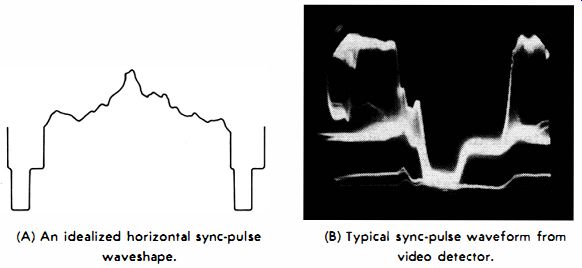
Fig. 7-7. Comparison of theoretical and practical waveforms. (A) An idealized horizontal sync-pulse waveshape. (B) Typical sync-pulse waveform from video detector.

WAVEFORM DETERIORATION

When a waveform is processed through successive circuits, progressive deterioration is inescapable. The technician's task is to distinguish between tolerable and abnormal waveform deterioration. Beginners who are schooled in theory alone sometimes expect to observe theoretically correct waveforms in electronic circuits. However, substantial departures from theory may be tolerable and satisfactory from the standpoint of practical operation. Fig. 7-7 illustrates these practical considerations of tolerance for a sync-pulse waveform. Not only does the practical waveform display slope and tilt, but it is also mixed with residual AC voltages from the receiver circuits.

More significant than the niceties of waveshape in this case is the relative amplitude of the sync tip to the complete video-signal excursion. The sync tip normally comprises 25% of the peak-to-peak signal voltage. Suppose, however, that overload in the IF amplifier compresses the sync tip to 10% of the peak-to-peak signal voltage. This is a serious distortion from a practical viewpoint, because the output from the sync separator will be attenuated. In turn, horizontal sync action will be unstable or completely lost. Accordingly, the relative amplitude of a waveform can be more important than its exact waveshape in some instances.

Reference Video Waveform

Note that amplitude observations of sync are made with respect to the total excursion of the video signal, which in turn changes greatly from time to time. Unless peak whites are present in the scanned scene, the peak-to-peak voltage of the complete video signal is less than maximum. Furthermore, due to lack of close tolerances on some transmissions, the sync tip may not appear at correct amplitude even when there are peak whites in the camera signal. Hence, it is better to use a pattern generator in such analyses-making certain, of course, that the pattern generator is in proper adjustment.

WAVEFORM CONTAMINATION

A certain amount of contamination by noise and residual AC voltages must be expected in most waveforms; however, the contamination must not be excessive. Your guide in this area consists of the key waveforms published in receiver service data-these are photographs of operating waveforms in a normal chassis. Thus, if you observe an abnormal amount of hum interference, for example, in an otherwise normal waveform a circuit defect is indicated. The hum interference could be due to a defective filter capacitor in the power supply or a tube that has developed heater-cathode leakage.

In the case of hum interference in a waveform, you will often find it helpful to evaluate the hum frequency. If you find it is 60-cycle hum, the most likely cause is heater-cathode leakage in a tube. But if you find it is 120-cycle hum, the most likely cause is inadequate power-supply filtering. To distinguish between the two cases, observe the video signal at a 60-cycle (or 30-cycle) deflection rate. Vertical-sync pulses occur at 60-cycle intervals; thus, it is easy to see whether the sync pulses are riding on a 60-cycle voltage or on a 120-cycle voltage.

Fig. 7-8 shows a typical example of 60-cycle hum voltage in a video signal. Note how the horizontal sync pulses "ride" on the hum voltage. The hum voltage is not a pure sine wave--it consists of a 60-cycle fundamental with considerable even-harmonic content. The reason for this particular waveshape is that the hum voltage is a ripple waveform from a half-wave power supply. On the other hand, when hum voltage stems from heater-cathode leakage, it has a fairly good sine waveshape, unless the tube operates in class B, such as a heterodyne mixer or video-detector tube. Thus, hum voltage in a video waveform must be evaluated with respect to the circuitry utilized in the power supply and in the affected sections of the receiver.

Hum Modulation of Video Signal

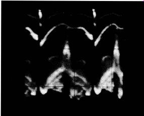
Fig. 7-8. Video signal with 60-cycle hum.

Observe also in Fig. 7-8 that the hum voltage modulates the amplitude of the horizontal sync pulses. To put it another way, the sync pulses are comparatively low in the center of the camera signal (where the hum voltage rises to its crest) , and comparatively high near the vertical-sync interval where the hum voltage falls to its minimum value. This hum modulation is the result of changing plate and screen voltages (and also cathode bias), due to the rise and fall of the ripple voltage. To put it another way, the gain of the affected stages varies with the amplitude of the hum voltage.

The same symptom is observed if there is hum voltage present in the AGC section-the bias level on the RF and IF stages rises and falls with amplitude of the hum voltage. In turn, the video signal becomes modulated at the hum frequency. In case of doubt as to the source of hum modulation, you can clamp the AGC line with battery bias or by means of a bias box. The possibility of hum modulation from the AGC section is thereby eliminated, which helps to identify the section where modulation is occurring. If the hum modulation persists when the AGC line is clamped, trace the distorted signal back through the signal channel to find where it first appears.

Horizontal-Sync Attenuation

Another aspect to be considered in the waveform of Fig. 7-8 is the depression of the horizontal-sync level below the vertical sync level. This means that there is a high-frequency attenuation present (horizontal sync pulses occur 15,750 times per second, while vertical sync pulses occur 60 times per second) . Do not jump to the conclusion, however, that the high-frequency attenuation is necessarily being caused by a circuit defect-the scope may be loading the circuit and impairing its high-frequency response. A low-capacitance probe must be used instead of a direct cable in video circuitry to avoid this difficulty. Even when a low-C probe is utilized, the normal action of peaking coils may be disturbed. Hence, for a definite test, apply the low-C probe at a low-impedance point in the video amplifier, such as across the contrast control.

SYNC SEPARATION

Another discrepancy between theory and practice is illustrated for a sync separator in Fig. 7-9. In theory the output from a sync separator consists of ideally rectangular pulses, but in practice the output has a characteristic spike shape. The reason for this departure is that the incoming sync tips have sloping sides, as previously explained. Furthermore, the tube does not have an ideally sharp cutoff characteristic, which tends to broaden the base of the output. The applied sync tips drive the grid into current flow, and hence the grid operates with a signal-developed bias. Previous discussion has pointed out how grid-current limiting tends to round the top of a pulse, even if the applied waveform has a perfectly flat top-the grid resistance characteristic is non-linear.

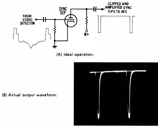
Fig. 7-9. Sync separator waveforms. (A) Ideal operation. (B) Actual output waveform.

This is another example of a situation in which the shape of the output waveform is of almost no concern; the important consideration is whether the amplitude of the output pulses is normal. On the other hand, if you observe spurious AC in the output waveform, there is a defect present which causes an in correct clipping level, and the spurious components can disturb or completely upset normal AFC action. Fig. 7-10 shows a typical waveform which contains objectionable interference, due to an incorrect clipping level.

You will find variations in tolerances of interference, depending on individual receiver designs-some AFC systems are more tolerant of residual video than others. The important point is to check the receiver service data in each case to determine whether the interference level is a matter for concern.

Otherwise, a false evaluation could be made which would lead to a waste of time in looking for a defect in the wrong place.

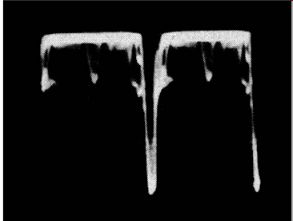
Fig. 7-10. Output from a sync separator when clipping level is incorrect.

COLOR-BURST WAVEFORM

Another interesting example of a discrepancy between theory and practice is shown in Fig. 7-11. Beginners who are familiar with theory only might expect to see a clearly defined and squared-off color burst at the output of the video detector.

Actually, the burst almost always has a slow rise and fall, as seen in the photo. Furthermore, the structure of the burst is seldom apparent on a service-type scope, because the 3.58-mhz sine wave is mixed with various interference components, and because it is difficult to synchronize the scope with the burst frequency.

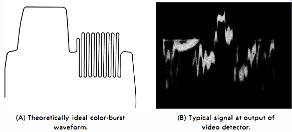
Fig. 7-11. Color-burst waveform. (A) Theoretically ideal color-burst waveform. (B) Typical signal at output of video detector.

WHEN WAVESHAPE IS IMPORTANT

It must not be assumed from the foregoing examples that waveform amplitude is always a dominant consideration over wave shape. Quite to the contrary, you will encounter many practical situations in which waveshape is the chief point of concern, and amplitude is incidental. Recall that when an amplifier is tested for amplitude distortion, only the shape of the pattern comes in for critical examination-the pattern amplitude is beside the point. A case in point is shown in Fig. 7-12.

This is the grid waveform of a burst-amplifier tube when the color receiver is energized by a keyed-rainbow signal.

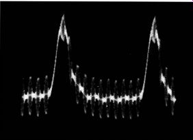
Fig. 7-12. Input to burst amplifier.

Circuit action here is the chroma counterpart of the sync-separator principle which was illustrated in Fig. 7-9. In other words, the sync separator in a receiver picks out the sync tips from the video signal, while the burst amplifier in a color receiver picks out the burst from the complete chroma signal.

Burst separation is accomplished by operating the burst amplifier tube beyond cutoff, except for the brief horizontal flyback interval, during which time the tube is driven into conduction. A suitably timed pulse from the horizontal-sweep system is applied to the cathode of the burst-amplifier tube to make it conduct during flyback.

Thus, the grid waveform shown in Fig. 7-12 displays the complete chroma signal riding on the cathode-keying waveform. As the keying waveform rises to its peak, the tube comes out of cutoff. The burst signal rides on top of the keying peak, and the burst is separated from the chroma signal and amplified in the plate circuit of the burst amplifier. It is clear that the burst must be seated on top of the keying pulse, and this is the point of first concern when tracking down the cause of poor color sync or complete loss of color sync. Otherwise stated, if the timing of the keying pulse is incorrect, it is beside the point to make any amplitude checks until after correct timing is restored.

Note in passing that incorrect timing can result from defective capacitors in the keyer circuit, resistors which may have increased considerably in value, or leakage from the keyer winding to the core in the flyback transformer. AFC trouble can also cause poor timing in some receivers, because when the horizontal oscillator is pulling strongly, the keyer pulse can be delayed or advanced, as the case may be. Note also that the series of bursts which appear along the pattern in Fig. 7-12 are arbitrary and result from the use of a keyed-rainbow generator in the timing test. If you use an NTSC generator, for example, the bursts will not appear, but instead you will observe a series of chroma bars--usually six bars, although some generators supply only one bar at a time. However, the colorburst display on top of the keying pulse is always the same, regardless of the signal source utilized.

Shape of Response Curve

Another important example of a situation in which waveshape is of central concern, while amplitude is incidental is shown in Fig. 7-13. This is the IF -response curve of a color receiver. In this particular design, the 3.58-mc chroma subcarrier and its sidebands are passed through the IF strip on the flat top of the frequency-response curve. Alignment is quite critical in this case. If the bandwidth of the response curve is too narrow, the color signal falls on the side of the curve, and some of the chroma sidebands may even be lost along the baseline, where the output is zero.

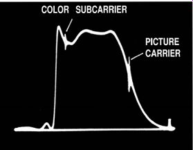
Fig. 7-13. IF response curve of color·TV receiver.

When this happens, the color signal is weakened and distorted. Color reproduction is poor, and if the bandwidth is abnormally narrow, color sync is also lost. Thus, variations in response-curve shape which would be of minor concern in black-and-white receivers assume great importance in this type of color receiver. This is not to say that IF alignment is equally critical in all color receivers-many utilize vestigial chroma sideband response, in which the chroma signal falls on the side of the response curve by design. While the IF adjustments are somewhat less critical in this type of receiver, it is nevertheless necessary to make certain that the 3.5S-mc subcarrier is not attenuated more than 6 db. Otherwise, the available gain in the subsequent chroma circuitry will be inadequate to obtain satisfactory color intensity.

When vestigial chroma-sideband response is employed, alignment of the following bandpass-amplifier section becomes some what critical, because a suitably tilted top must be provided by the response curve to compensate for the slope in the chroma region of the IF curve. If this complementary waveshape is not observed, the chroma sidebands become distorted, which in turn deteriorates the color reproduction. In any case, your safe guide to correct waveshapes is the service data for this particular receiver.

Phase Distortion

Phase distortion must sometimes be evaluated in frequency response curves, as well as in square-wave patterns. An example is shown in Fig. 7-14. Fig. 7-14A shows a response curve in which trace and retrace layover is good. On the other hand, Fig. 7 -14B shows very poor layover due to phase distortion in the test setup. When you see a situation of this sort, it is point less to blank out the retrace or to convert it to a zero-volt base line, because the phase distortion is changing the shape of the curve and will lead to false conclusions. The source of the phase distortion must be localized and eliminated.

A common cause of this difficulty is shunting of excessive capacitance across the scope vertical input terminals. Another possibility is the use of an excessively large isolating resistance in series with the vertical input lead of the scope. Technicians commonly employ an isolating resistor and/or a shunt capacitor across the scope input terminals to sharpen the marker indication and suppress interference on the response curve. As long as the time-constant of the combination is not excessive, negligible phase distortion is introduced. However, too long a time constant leads to the difficulty illustrated in Fig. 7-14. Rarely, a defect in the sweep generator produces similar pattern distortion.

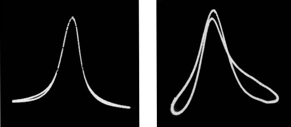
Fig. 7-14. Frequency-response displays. (A) Negligible phase distortion. (B) Severe phase distortion.

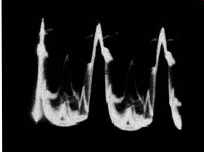
Fig. 7-15. Effect of narrow IF bandpass on sync-pulse waveform.

BANDWIDTH VERSUS SYNC-PULSE REPRODUCTION

Sync-pulse waveforms and amplitudes become changed when the circuit bandwidth is subnormal. The amplitude change is best observed with 30-cycle scope deflection, as was illustrated in Fig. 7-8. Wave shape change can be observed with 7,875-cycle deflection, as shown in Fig. 7-15. As the circuit bandwidth is made narrower, the sync pulses become more extensively integrated, or "feathered". It is possible to be misled, however, unless you energize the receiver from a test-pattern generator which has close-tolerance sync. The reason for this requirement is that station-signal sync is often deteriorated to some extent.

Network programs in particular often have substandard sync. However, if you use a good-quality pattern generator, the sync pulses have a fast rise and flat tops. Thus, the sync pulses provide the facility of a square-wave test in evaluating the circuit action. While the evaluation is limited to 15,750-cycle pulse response, it will nevertheless be quite informative, provided that you are using a good pattern generator. Subnormal band pass always reduces picture quality-the first question which arises is whether the narrow bandpass stems from the IF amplifier or video amplifier; inasmuch as tuner response curves are usually quite broad, the trouble will usually be localized in either the IF amplifier or the video amplifier.

For example, if you find a video waveform such as shown in Fig. 7-15 at the output of the video amplifier, transfer the low-C probe back to the video-detector output. If you find a normal video signal at the detector, the trouble is in the video amplifier. On the other hand, if the same distortion appears at the detector, the trouble is in the IF amplifier. Suppose that your pattern generator does not have fast-rise and flat-topped sync pulses-then evaluation of pulse shape is beside the point.

However, you can approach the problem from another view point, by making the generator supply sharp pulses. All that is necessary is to insert a white-dot slide instead of a test-pattern slide into the generator. Then the scanner automatically generates sharp pulses which are well suited for bandwidth evaluation.

Distortion of the pulses by narrow-bandwidth circuits can be evaluated on the basis of amplitude. Although the pulses are broadened when they pass through a narrow-band circuit, this effect is much less apparent than the reduction in amplitude.

Thus, at the output of the generator, the sync tips will normally have 25% of the total waveform amplitude. If you check at the output of the video amplifier and find that the sync tips now have a different amplitude, it is evident that the signal has passed through a circuit with subnormal bandwidth. Transfer the low-C probe back to the video-detector output. This will immediately show you whether the trouble is in the IF amplifier or the video amplifier. Of course, you will encounter chassis in which both the IF amplifier and video amplifier have sub- normal bandwidths. In such case, the pulse amplitude is reduced by passage through the IF amplifier and further reduced by passage through the video amplifier.

White-dot Signal Generator

It is apparent that a test-pattern generator with a white-dot slide is of great utility in practical test work. Not only does it provide a steady and controllable signal, but the availability of a white-dot slide provides the facility of a high-performance square-wave generator. Why do we not use an ordinary test pattern signal when localizing narrow bandwidth in a chassis ? It is true that a test-pattern signal contains high-frequency video information, but the high-frequency data in a test-pattern signal tends to be obscured by low-frequency data, whereas in a dot signal the high-frequency components are clearly in evidence. Although an experienced operator can work with the high-frequency components in a test-pattern signal, the beginner is better advised to utilize a dot signal in this type of test work.

COLOR-BAR SIGNAL IN BLACK-AND-WH ITE TESTS

If you have a color-bar generator available, the color signal provides the equivalent facility of a dot signal for localization of narrow bandwidth. For example, consider the signal illustrated in Fig. 7-16. This is a mixed waveform with fundamental frequencies of 15,750 cycles and 3.58 mhz. A black-and-white receiver in good operating condition has substantial response at 3.58 mhz. This signal was applied to a high-quality black-and-white receiver, and the 3.58-mc component was attenuated about 10% at the video-detector output. This is quite acceptable performance. Suppose you should find that the color bars were attenuated to 50% of their normal amplitude in this test-it is then indicated that the IF amplifier is in need of realignment.

This check can be repeated at the video-amplifier output to determine whether high-frequency attenuation is occurring in this section of the receiver. In most cases, poor high-frequency response in the video amplifier will be tracked down to load resistors which have increased in value. Remember that the video-detector load resistor is a part of the video-amplifier system. If it increases in value, high video frequencies will be attenuated. If the load resistors have correct values, the next most likely culprit is an off-value or defective peaking coil.

Peaking-coil values are rather critical-a point which is usually overlooked by beginners.

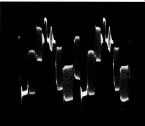
Fig. 7-16. Color-bar signal at output of video detector.

It should be unnecessary to point out that the resistance of a peaking coil has no necessary relation to its inductance.

The critical parameter of a peaking coil is its inductance, and this cannot be measured with an ohmmeter. Unless you have an impedance bridge available, a suspected peaking coil should be checked by substitution. Always refer to the receiver service data for specifications of correct replacements. In case poor high-frequency response is not due to defective peaking coils, check out the decoupling circuits in the video amplifier.

PEAK-TO- PEAK VOLTAGES VERSUS DC VOLTAGES

There is no necessary relation between the DC voltage and peak-to-peak voltage in an electronic circuit. It is perhaps surprising to the beginner to find that a peak-to-peak voltage may be less than, equal to, or greater than the DC voltage at the test point. For example, the plate-supply voltage to a horizontal output tube might be 420 volts DC. But the peak-to-peak voltage of the plate waveform might be 6,000 volts. Where does this extra voltage come from? It stems from the stored energy in the cores of the Flyback transformer and yoke. When the horizontal output tube is suddenly cut off, a counter-emf, or kickback, voltage is generated which greatly exceeds the DC operating voltage.

TROUBLESHOOTING BY WAVEFORM ASPECT

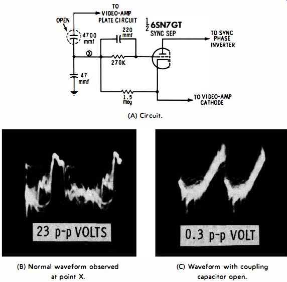
Fig. 7-17. Use of waveforms to locate circuit defect. (A) Circuit. (B) Normal waveform observed at point X. (C) Waveform with coupling capacitor open.

Most troubleshooting procedures involve changed waveform aspects, although amplitudes are also important. An example is illustrated in Fig. 7-17. The initial symptom is loss of horizontal sync. DC voltage and resistance measurements in this situation do not help to pinpoint the defective component (an open coupling capacitor) . However, when the video signal is traced through the sync circuitry, a different waveform is observed on either side of the 4700-mmf coupling capacitor. In normal operation, there would be practically no change of waveform across the capacitor. The amplitude of the distorted waveform on the output side of the capacitor is also very low.

Thus, the waveform analysis points directly to an open capacitor. It might be supposed that no signal at all would be found on the output side of the capacitor. However, a small transfer does take place because of stray capacitances. Moreover, when the coupling capacitor is open, the grid network of the sync-separator tube becomes a high-impedance circuit. In turn, the grid circuitry picks up a substantial amount of stray field voltage, which contributes to the 0.3-volt p-p waveform which is observed. In other words, the abnormal waveform is not merely a sharply-differentiated and attenuated version of the normal waveform, but also contains stray-field components.

Waveform analysis is the only practical way to localize open capacitors in many cases, because there is often no significant DC voltage or resistance change. Accordingly, without waveform information there is no way to localize the trouble area.

INTERFERENCE PICKUP VERSUS CIRCUIT IMPEDANCE

One of the more sophisticated aspects of distortion analysis concerns waveform change due to impedance variation. An example is illustrated in Fig. 7-18. Note how the interference level at the cathode of the clipper increases enormously when , the 100-mmf coupling capacitor is open. This rise in the interference level is accompanied by a reduction in peak-to-peak voltage. If you analyze the distorted waveform, you will deduce immediately that the 100-mmf coupling capacitor must be open, because the interference can only stem from the grid circuit stray fields can induce appreciable voltage in high-impedance circuits only.

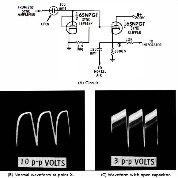
Fig. 7-18. Change of waveform due to change in impedance. (A) Circuit. (B) Normal waveform at point X. (C) Waveform with open capacitor.

It is not always recognized that the value of a coupling capacitor can determine the input impedance of a grid circuit. However, this is easily understood if the coupling capacitor is regarded as a bypass capacitor. This is so because the output of a sync-amplifier has only moderate impedance. Thus, with respect to the high-resistance grid return (3.9-megohms), the 100-mmf coupling capacitor can be regarded as grounded at its input end. So far as stray pickup is concerned, the grid input impedance is equal to the reactance of the coupling capacitor.

When the coupling capacitor is open, the input impedance of the grid circuit becomes 3.9 megohms, and the stray fields will induce more interference voltage in the grid circuit. The result is a very large increase in the interference level. The abnormal waveform does not consist entirely of interference voltages, but a small amount of stripped sync is also passed because an "open" capacitor still has a small residual capacitance.

Thus, the trouble waveform in Fig. 7-18, which has a baffling structure to the inexperienced operator, tells its story of impedance variation and induced stray-field voltage to the technician who has learned how to analyze distorted waveforms.

This knowledge is founded on an understanding of basic electronics and circuit action. In summary, you must understand circuit theory in order to read out the information displayed in an unusual waveform.