Waveform Measurements [Scope Waveform Analysis (1963)]

Some waveform measurements are obvious; for example, since a scope is basically a voltmeter, vertical deflection is directly proportional to peak-to-peak voltage. Since the voltage across a resistor is proportional to current, vertical deflection is directly proportional to peak-to-peak current when the waveform is taken across a resistor in a circuit. On the other hand, measurement units that are not proportional to vertical deflection are not entirely obvious. Decibel measurements are a case in point.

HOW TO MEASURE DB WITH A SCOPE

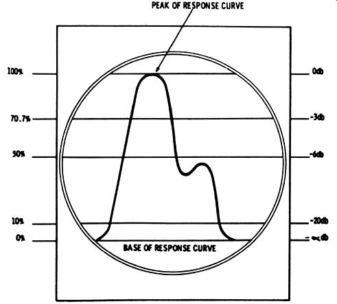
Fig. 6-1. Correlation of db response and percentage response.

It is often necessary to identify various db points on a frequency-response curve. If the bandwidth of a TV-IF curve is defined as the frequency interval between the -6 db points on the curve, this simply refers to the points half way down from the peak of the curve to the base line. A trap response might be specified as -20 db down, which means a point 90% down on the response curve.

Decibels can be defined in terms of vertical deflection in this manner because the scope is connected across the same load for all db measurements taken on any one curve. It makes no difference what the load may be because the difference between db readings across any fixed load is a true measurement that requires no conversion. The derivation of this relation is not of present importance, but its availability permits the construction of direct-reading db graticules for scopes (Fig. 6-1) . A db graticule is employed only in specialized applications which require a long series of db measurements. Usually an ordinary graticule is used, and reference is made to a table of voltage ratios versus db values when db readings are being made.

Dual db Scales

On IF and RF frequency-response curves, measurement is always made in terms of db loss. In other words, the peak of the curve is taken as the reference point (0 db) , and all measured db values are negative. When evaluating the response of an audio amplifier, it is customary to take the gain at 1,000 cycles as the 0-db reference point; the gain at other frequencies may be either greater or less than 0 db. Hence, graticules employed in this type of test are provided with two db scales, one of which is calibrated in db gain and the other in db loss. In specifying the total variation of an audio-frequency response curve, the maximum and minimum values are read, for example, ±3 db, or +2 and -4 db. The practice of analyzing frequency-response curves in terms of db loss and db gain with respect to a mid-band 0-db reference extends to wide-band amplifiers, such as TV -distribution amplifiers.

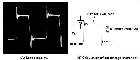
Fig. 6-2. Overshoot and ringing. (A) Scope display. (B) Calculation of percentage overshoot.

PERCENTAGE OVERSHOOT

Amplifiers are often rated for overshoot at a specified square-wave frequency. For example, an amplifier might be rated for less than 10% overshoot when driven by a 10-khz square wave.

The meaning of percentage overshoot is shown in Fig. 6-2B. In this example, overshoot is followed by ringing-this is often the case, although overshoot occasionally occurs without subsequent ringing. In Fig. 6-2A overshoot occurs on the trailing edge as well as on the leading edge. The trailing overshoot may have the same percentage as the leading overshoot or a different value. In some cases, overshoot occurs only on ' one edge.

An amplifier may develop overshoot without ringing on the leading edge or overshoot on the trailing edge. Both positive and negative peaks may exhibit tilt. An overshoot may terminate quickly or gradually; in the limit, the overshoot becomes a tilt. Intermediate situations can be characterized as either a prolonged overshoot or as tilt with curvature. Percentage tilt is measured in the same manner as percentage overshoot.

Amplifier square-wave responses often show a combination of characteristics, such as overshoot with ringing, overshoot with tilt, or overshoot with ringing and tilt. When overshoot is tolerated, it is the price paid for faster rise time. In other words, most amplifiers provide decreased rise time if a reasonable percentage of overshoot is permitted. If residual inductance is present in the amplifier circuitry, the overshoot is usually accompanied by ringing. Whether ringing is brief or prolonged depends on the Q of the associated inductive circuit. This fact is put to use to measure the Q of the coil. If you measure the ringing frequency, you can also find the inductance and the AC resistance of the coil under test.

HARMONICS AND RINGING FREQUENCY

In most cases the ringing frequency has no relation to the fundamental or harmonic frequencies of the distorted square wave. Hence, when it is desired to measure the ringing frequency, this procedure may be carried out without regard to the square-wave repetition rate. To measure a ringing frequency, first adjust the scope controls so that the ringing interval occupies an appreciable portion of the screen area. This gives ample excursion of the ringing waveform so that it can be effectively analyzed. Then, note the number of horizontal squares occupied by one cycle of the ringing waveform. This number of squares is used for reference in the final step of the procedure. Disconnect the scope from the source of the ringing waveform and feed the output from an audio oscillator into the scope. Without changing the settings of the scope controls, adjust the audio-oscillator tuning control until the number of horizontal squares observed previously is occupied by one cycle. The reading of the dial on the oscillator then gives the ringing frequency. Note that ringing intervals are often encountered when any complex waveform is applied to the input of an amplifier.

ANALYSIS OF ODD AND EVEN HARMONICS

Whether a complex waveform contains odd harmonics only, even harmonics only, or both odd and even harmonics can be seen from the mathematical expression for the waveform. Thus, a square wave can be expressed by the equation:

4E e = -(cos cut - 7? cos 3 cut + 7f % cos 5 cut - ? cos cut . . .) where, e is the instantaneous voltage, E is the peak voltage, cu is 6.28 times the fundamental frequency.

This is called the cosine expression of a square wave. Any desired number of cosine terms can be added to the equation.

A cosine wave has the same shape as a sine wave, but it differs 90° in phase. A minus sign in the expression means that the harmonic is 180° different in phase from the same harmonic with the plus sign.

It is obvious that the frequencies in a square wave are related according to factors of 1, 3, 5, 7, 9, 11, etc. Hence, a square wave contains odd harmonics only. The ringing frequency in Fig. 6-2 is a new and arbitrary frequency which is added to the harmonic frequencies contained in the reference square wave.

The ringing frequency can be filtered out by a harmonic analyzer, just as a harmonic of the reference square wave can be filtered out.

Output of Full-Wave Rectifier

Compare the expression for a square wave with that for the output from a full-wave rectifier; the succession of half-sine waves from a full-wave rectifier is described by the expression: e = 2E (1 + % cos 2cut - 715 cos 4 cut + %5 cos 6 cut - .... ) 7f where, e is the instantaneous voltage, E is the peak voltage, cu is 6.28 times the fundamental frequency.

The frequencies are related according to factors of 2, 4, 6, 8, etc.; the wave contains even harmonics only. Compare the foregoing expressions with that for a sawtooth wave:

e = 2E (sin wt - % sin 2wt + Y:J sin 3 wt - Y4 sin 4 wt ... )

.". where, e is the instantaneous voltage, E is the peak voltage, w is 6.28 times the fundamental frequency.

The frequencies in a sawtooth wave are related according to factors of 1, 2, 3, 4, etc. Accordingly, a sawtooth wave contains both even and odd harmonics. Any expression of sines can be converted to cosines, or vice versa, but, of course, the harmonic relations described are the same.

Pulse With Infinitesimal Width

When you differentiate or integrate a waveform, the frequencies of the harmonics are unchanged; however, their amplitudes and phases are changed. Suppose an ideal pulse is integrated and a square wave is obtained. This shows that a pulse contains the same frequencies as a square wave. Next, suppose that the square wave is integrated; a pyramid (back-to-back sawtooth) wave results, and it is evident that the same harmonic frequencies are present. If this wave is integrated, a parabolic wave is obtained, and the same harmonic frequencies are present.

An ideal impulse wave contains odd harmonics only, and each harmonic has the same amplitude. Integration weakens the higher harmonic amplitudes so that the third harmonic in the resulting square wave has 1/3 the amplitude of the fundamental, the fifth harmonic has 1/5 the amplitude of the fundamental, etc. If you integrate the square wave to form a pyramid wave, the higher harmonic amplitudes are weakened still more.

The expression for a pyramid wave is:

8E e = - (cos wt + 1/9 cos 3 wt + 1/25 cos 5 wt + .. .. )

.".2

where,

e is the instantaneous voltage,

E is the peak voltage,

w is 6.28 times the fundamental frequency.

When you integrate the pyramid wave to obtain a parabolic wave, the harmonics decrease in amplitude still more rapidly.

The succession of parabolic waves looks very much like a sine wave, and indeed, if an infinite number of integrations is carried out, you would arrive at a pure sine wave having the frequency of the fundamental, since all harmonic amplitudes would ultimately become zero.

Note that you can go backward from a parabolic wave and by successive differentiations arrive at an impulse wave. In this case each differentiation brings up the amplitude of the higher harmonics.

When a waveform is expressed mathematically, it is said that the analytic solution has been obtained. In a sense, then, a scope is an analog computer.

Q VALUE OF A COIL

A distinction must be made between two different types of Q values for a coil. The basic value is the Q of the coil in isolation, i.e., when it is not loaded by associated circuitry. The other value of Q is lower for the same coil. It is obtained when the coil is loaded by various circuit components to which it may be connected, such as in an amplifier. Ringing patterns provide a convenient means of measuring the Q of an isolated coil. When you connect the coil to the input terminals of a scope, the coil is isolated for all practical purposes because the input impedance of a scope is very high. The stray capacitance that is present will resonate with the coil at some frequency.

A pulse voltage is injected into the coil by very loose coupling. For example, some scopes have a front-panel terminal which supplies a pulse voltage; connect a lead to the pulse terminal and place the open end of the lead near the coil. This provides very loose capacitive coupling. Now, a damped sine wave should appear on the scope screen (Fig. 6-3) . Note the points indicated at a and b in Fig. 6-3. At b, the amplitude of the damped sine wave has decreased to 37% of its amplitude at a. In other words, if there are 16 squares of vertical deflection at a, there are 6 squares at b. The significance of the 37% value is that it shows the time constant of the ringing coil.

The Q of the coil is given by the formula:

... where, pi is 3.1416, n is the number of peaks between a and b.

Q in this example is approximately 22.

If you know what the Q value of a coil should be, you can make a ringing test to check the Q value. Shorted turns, for example, reduce the normal Q value. This is merely a simple comparison test, and additional waveform observations must be made to obtain a more complete evaluation of the coil.

These are discussed subsequently, but now, consider how you would measure the Q of a coil which is connected in a resonant circuit.

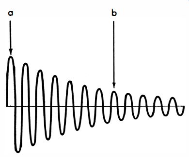
Fig. 6-3. Determination of Q from ringing waveform.

It is most convenient to determine the Q of the loaded coil by evaluating the frequency-response curve for the stage (Fig. 6-4) . This is done by noting the frequencies at the -3 db points on the curve. The -3 db points occur at 70.7% of peak amplitude-they are often called the half-power points. The Q of the loaded coil is then given by the formula:

Q = fr / f2 - f1

where,

fr is the center frequency,

f1 and f2 are the frequencies at the -3 db points.

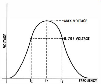
Fig. 6-4. Determination of Q from frequency response curve.

Ringing Frequency

The value of Q means little unless you specify the frequency at which it was measured. This lack of meaning results from the fact that the Q value changes with frequency. In Fig. 6-3 you would relate the Q value to the ringing frequency. How do you measure the ringing frequency? If the scope has calibrated horizontal sweeps, you can read the frequency from the ringing pattern. However, most scopes do not have calibrated sweeps, and an audio oscillator is required. Connect the output from the audio oscillator in place of the coil and adjust the frequency until the pattern shows the same number of peaks between a and b as before. The dial of the audio oscillator then indicates the ringing frequency.

AC RESISTANCE

Beginners sometimes suppose that the AC resistance of a coil is the same as its DC resistance. This is not necessarily true.

At low frequencies, such as 60 cycles, the AC and DC resistances are practically the same for most coils. On the other hand, at higher frequencies, such as 1 mhz, the AC resistance will always be higher-often very much higher-than the DC resistance. It is easy to measure the AC resistance of a coil at its ringing frequency. Merely connect a potentiometer in series between the coil and a tuning capacitor (Fig. 6-5) . The tuning capacitor may be adjusted for any desired ringing frequency within its range.

The potentiometer is used to determine the AC resistance of the coil. To do this, note that the ringing waveform becomes more highly damped and dies out faster when the value of R (Fig. 6-5) is increased. Referring to Fig. 6-4, the ringing waveform falls to 37% of its initial amplitude after 7 peaks. If you adjust the potentiometer so that the waveform falls to 37% of its initial amplitude after 3% peaks, the resistance of the potentiometer is equal to the AC resistance of the coil. You can measure the potentiometer resistance with an ohmmeter.

Fig. 6-5. Method of determining AC resistance of a coil.

The value of AC resistance changes with the ringing frequency; hence, a measured value of AC resistance should be stated with respect to the frequency at which it was measured.

In general, the higher the ringing frequency, the higher is the AC resistance. In this respect, Q values and AC resistance values are both functions of frequency-other things being equal, Q doubles when the frequency is doubled. However, other things are seldom equal, because the AC resistance varies with frequency in a more or less unpredictable way. Inasmuch as Q depends on both frequency and AC resistance, it is evident that a Q measurement at one frequency does not justify a prediction of its value at some other frequency.

Inductance

If you have measured the ringing frequency and the Q and AC resistance at this frequency, the inductance of the coil can be determined by the formula: where, L is the inductance in henrys, Q is the quality factor at frequency f, f is the ringing frequency in cycles per second, pi is 3.1416.

The henry, of course, is a large unit of inductance, and most of the coils commonly used in electronic circuits have inductances in the millihenry (0.001 henry) range. If you express f in kilocycles, then L is given in millihenrys in the foregoing formula.

The inductance of an air-core coil is practically constant at any frequency of operation. On the other hand, a permeability tuned coil may have quite different inductance values at different frequencies; this change in inductance stems from different characteristics of the powdered core material at various frequencies. Note that the inductance of coils with laminated iron cores, such as output transformers, will have less inductance when the current flow is heavy. This results from partial saturation of the iron. Thus, plate-current flow through the primary of an output transformer reduces its effective inductance.

UNTUNED TRANSFORMER

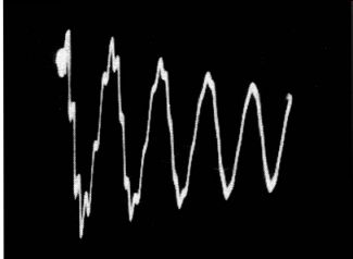
Fig. 6-6. Ringing waveform of a transformer winding.

Untuned transformers, such as flyback transformers, exhibit highly complex ringing waveforms in some cases. A typical pattern is shown in Fig. 6-6. Although a transformer is regarded as untuned in the sense that tuning capacitors are not connected across the windings, capacitance is nevertheless present. There is distributed capacitance between layers of the windings, with the result that the windings have self-resonant frequencies.

The various windings are also coupled rather tightly by the ferrite core so that a complex electrical system results. Because the situation is so involved, ringing tests are usually made on a comparative basis only.

When a flyback transformer is connected into a horizontal output circuit, the tendency to ring on forward scan is less than for an isolated transformer. The primary is loaded by the horizontal-output tube. At the end of the forward scan, the horizontal-output tube is suddenly cut off, and the flyback transformer, with its associated yoke circuit, rings strongly for one-half cycle. At the end of a half cycle, the damper tube conducts and heavily loads the secondary. In theory, no residual ringing would occur, but due to leakage reactances in the flyback transformer, more or less spurious ringing ensues. Thus, when you observe the screen-grid waveform, you often see evidence of spurious ringing (Fig. 6-7).

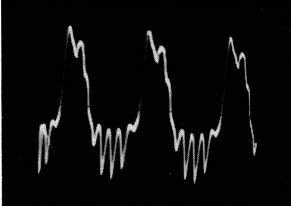
Fig. 6-7. Screen voltage waveform of a horizontal-output tube.

LEAKAGE REACTANCE

When primary and secondary are wound on the same core and coupled as tightly as possible (as in an output transformer) , there is no leakage reactance present, at least in theory. In other words, if the secondary terminals are short-circuited, it would be expected that the short would be reflected back to the primary terminals, and that the primary input impedance would be zero. In practice, the short circuit is less than 100% reflected to the primary, and you will observe more or less ringing when a pulse shock-excites the primary. There is a small amount of uncoupled inductance present, which is tuned to the ringing frequency by distributed capacitance. The residual ringing is said to be caused by the leakage reactance, which resonates with the stray capacitance.

Uncoupled inductance stems from stray magnetic field flux.

In other words, most of the flux set up by the primary threads through the secondary, but a small amount of flux fails to do so, escaping via air paths. Well designed output transformers have a very small amount of leakage reactance. On the other hand, a tuned IF transformer has a very high value of leakage inductance. The looser the coupling between primary and secondary, the greater is the amount of leakage inductance that exists.

DELAY TIME

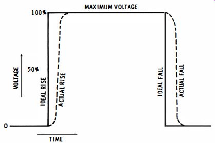
Fig. 6-8. Waveform showing 50% point.

In checking out delay lines and various special-purpose electronic devices, it becomes necessary to measure delay time. This is an input-output relationship and is defined as the elapsed time from the 50% point on the input waveform to the 50% point on the output waveform (Fig. 6-8). To make this measurement, you must know how much elapsed time is represented by each horizontal interval along the graticule. It is not always necessary to use a sophisticated scope with calibrated horizontal sweeps; an ordinary scope can easily be calibrated for this purpose.

For example, you can connect the output from a signal generator to the vertical input terminals of the scope and tune the generator to 1 mhz. Then, adjust the scope controls so that the sine-wave pattern crosses each horizontal interval. Each successive horizontal division then represents an elapsed time of function of the scope-for example, a lead can be connected from the external-sync terminal of the scope to the output of the device under test. Observe the input waveform first, and note its 50% point on the graticule; next observe the output waveform and note its 50% point. The separation of the 50% points gives an indication of the delay time.

USE OF EXPANDED DISPLAY

(A) Display with sweep magnifier. (B) Expansion of detail on retrace.

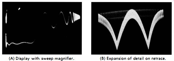
Fig. 6-9. Waveform expansion.

Various of the foregoing tests may be made on expanded sweep or triggered sweep, which can provide improved readability at high frequencies. Sweep magnifiers in lower-priced scopes do not always have a linear display; an example of poor linearity is shown in Fig. 6-9. A triggered-sweep function always provides as good linearity as free-running sawtooth sweep and may be preferred for this reason. You can display a ringing waveform as readily on triggered sweep as on conventional horizontal free-running deflection.

Scopes which do not have retrace blanking display a visible retrace, as shown in Fig. 6-9B. Since retrace is much faster than the forward trace, waveform detail is expanded on retrace.

This is the only possibility of waveform expansion on a simple scope, and it is sometimes helpful. However, a certain amount of skill is required to display the desired portion of the waveform on the retrace interval. Among the control considerations are employment of positive, negative, or external sync with close adjustment of the sync-amplitude and horizontal-frequency controls.

WAVEFORMS FOR LARGE INDUCTANCES

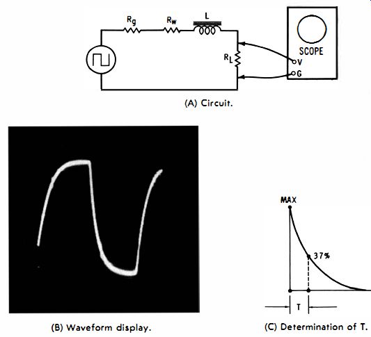
Fig. 6-10. Square-wave measurement of inductance. (A) Circuit. (B) Waveform display. (C) Determination of T.

Large inductances often have a low Q and will not ring when shock-excited; however, if ringing does occur, the damping is so rapid that satisfactory measurements cannot be made. Otherwise stated, the winding resistance is so high, and the distributed capacitance is so large (natural resonant frequency so low) , that the inductor is in the vicinity of or past critical damping; hence, other methods than ringing tests must be used to determine the inductance value. A square-wave test is convenient. An integrating circuit is used (Fig. 6-10) . The square wave generator is set to any convenient frequency which is low enough to produce a decay to practically zero (the end of each excursion is practically horizontal) . The inductance (L) in henrys is determined from the formula:

L= RTT

where, L is the inductance in henrys, T is the decay time in seconds, RT is the sum of Rg, Rw, and RL, Rg is the internal resistance of the generator in ohms, Rw is the winding resistance of ohms, RL is the load resistance in ohms.

Some generators have a rated output resistance, but if yours does not, it is easy to measure the output resistance (internal resistance). Simply connect a potentiometer across the generator output terminals and check the square-wave amplitude with a scope. When the output voltage drops to one-half the open-circuit value, the potentiometer resistance is equal to the generator internal resistance. At low frequencies, such as 100 cycles, Rw is practically the same as the DC resistance. Hence, measure Rw with an ohmmeter.

To measure T, note that this is the time for the waveform to fall from its maximum value to 37% of maximum. This is why the operating frequency should be chosen to obtain a flat top and bottom on the waveform-the pattern shows the level at which the waveform decays to zero. Locate the point 37% up on the decay curve by counting squares of vertical deflection.

Suppose you are operating the square-wave generator at 100 cycles. Then, the time for one complete cycle is 0.01 second.

If there are 10 horizontal squares included in one complete cycle, each square will represent 0.001 second. Merely count the horizontal squares from the start (maximum point) of the decay curve to the point where it has fallen to 37% of maximum. Multiplying the number of squares by 0.001 gives the value of T. The distributed capacitance of the inductor does not introduce appreciable error as long as the square-wave frequency is comparatively low. When the frequency is too high, you will not observe a waveform such as shown in Fig. 6-10, but instead a broken type of waveform will appear due to introduction of differentiation by the distributed capacitance. Therefore, always use a square wave frequency which gives a true integrated waveform. Note that the value of RL is not critical, and any value in the range of a few thousand ohms is satisfactory.

VIEWING TOTAL HARMONIC DISTORTION

When an amplifier distorts a sine wave, the output consists of the original sine wave plus the harmonics which have been generated. A scope connected at the output of the amplifier (Fig. 6-11A) shows the combined fundamental and harmonics (Fig. 6-11B) . The amplifier has distorted the input sine wave and made it unsymmetrical-the positive peak is broader than the negative peak. If the fundamental is filtered out (Fig. 6 11C) , the scope then displays the total harmonic distortion alone (Fig. 6-11D) . From the preceding discussion it would be anticipated that even harmonics have been generated by the amplifier. Fig. 6 11D shows that this is so; when the fundamental is filtered out by the harmonic-distortion meter, a double-frequency complex wave is displayed. This double-frequency characteristic shows that second-harmonic distortion is prominent. Of course, there are other harmonics present also, because the output from the harmonic-distortion meter is a complex wave and not a simple sine wave. The meter reads the percentage of total harmonic distortion.

Note that the output from the harmonic-distortion meter gives wave shape and frequency information only-it does not necessarily indicate either the polarity nor the phase of the total-harmonic-distortion waveform. Likewise, the relative amplitudes of the two waveforms in Fig. 6-11 are not given directly in this type of test-the test setup would have to be calibrated in order to measure the comparative amplitude of the distortion products. However, this is seldom necessary, because a related amplitude value is given by the reading of the harmonic-distortion meter.

MEASUREMENT OF DC COMPONENT

Whenever a waveform is passed through nonlinear resistance, it develops a DC component. An extreme example is a sine wave passed through a rectifier. A waveform across a cathode-bias resistor "rides on" the DC bias voltage. The waveform at the base of a transistor "rides on" the base-emitter DC voltage. This mixture of AC and DC voltages is displayed by a DC scope, as shown in Fig. 6-12A. Note that the sine wave is centered on the DC component. Since DC voltage is measured in the same units as peak-to-peak voltage, the DC component is determined by counting squares of vertical deflection.

(A) Scope connected to amplifier output. (B) Waveform at amplifier output. (C) Test setup to separate total harmonic distortion. (D) Waveform of separated distortion components.

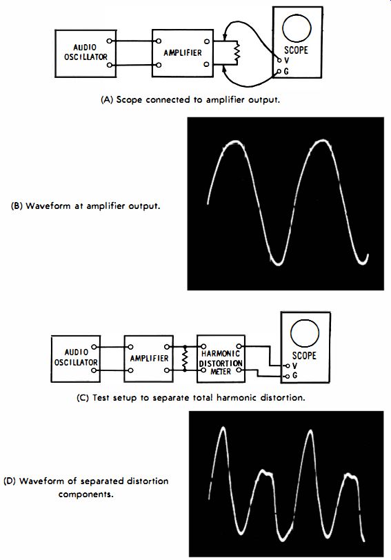
Fig. 6-11. Display of total harmonic distortion on a scope.

For example, if a scope is calibrated for a sensitivity of 1 volt peak-to-peak per square of vertical deflection, and the DC component level is located 10 squares above the base line, the value of the DC component is 10 volts. This is a comparatively simple example. The DC component level is readily apparent in Fig. 6-12A because a sine wave has a symmetrical form-in other words, the DC component level cuts half-way down the sine wave and divides it into equal positive and negative excursions.

(A) Sine wave superimposed on DC component. (B) Determination of DC-component level of complex waveform.

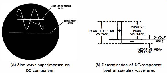
Fig. 6-12. Waveforms with DC components.

If you proceed to measure the DC component in a complex waveform, the DC component level may not be obvious. In such a case, first switch the scope to its AC function and note how the complex wave is placed above and below the 0-volt axis.

The waveform will be divided into equal areas. This division for a pulse wave is depicted in Fig. 6-12B. Next, switch the scope to its DC function-the waveform will rise on the screen (or fall if the DC component is negative). Now, note the separation between the former 0-volt level and the actual 0-volt level on the screen; this separation is a measure of the DC component. In other words, you do not have to guess where the DC component level cuts the waveform-a preliminary check on the scope AC function will give you this information.

Output From Demodulator Probe

There is always a DC component present in the output from a demodulator probe, because the probe contains a rectifier diode. The DC component provides convenient measurement of percentage modulation. For example, if you wish to measure the percentage modulation in the output signal from an AM generator, simply pass the signal through a demodulator probe into a DC scope. The demodulated envelope will then ride above the zero-volt level as in Fig. 6-12A. If the negative peaks touch the zero-volt level, the signal is 100% modulated. Over-modulation shows up as a clipping of the negative peaks.

Standard modulation for an AM generator is 30%. In this case the negative peaks dip 30% down from the DC component level toward the zero-volt level. You will find that the modulation percentage for an AM generator is not necessarily constant on different bands, nor even at different settings on the same band. Likewise, the modulation envelope is not always a true sine wave and in some cases changes shape considerably from one band setting to another. Hence, it is useful to have a quick check available for modulation percentage and waveshape. Note that the waveform might appear below the zero volt level, depending on the polarity of the diode in the demodulator probe.

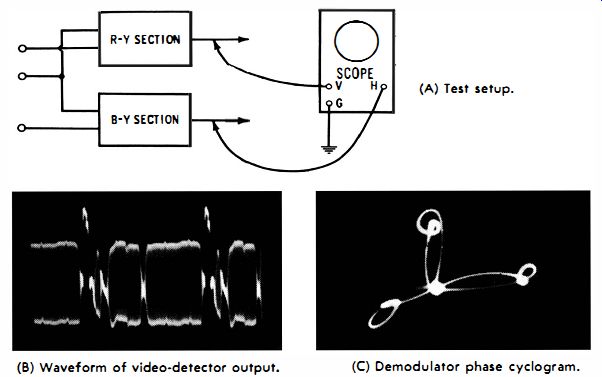
Fig. 6-13. Display of chroma phase information. (A) Test setup. (B) Waveform of video-detector output. (C) Demodulator phase cyclogram.

CHROMA-PHASE MEASUREMENT

Various types of waveforms are utilized to check and measure chroma-demodulator phases. The cyclogram (vectorgram) display shown in Fig. 6-13C is one type. To obtain the cyclogram pattern, the output from the R-Y section is connected to the vertical input terminals of the scope, and the output from the B-Y section is connected to the horizontal-input terminals. The color receiver is energized by a chroma signal from a color-bar generator comprising sync-and-burst, R-Y, and B-Y signals, as seen in the video-detector output waveform in Fig. 6-13B. The cyclogram shows the phases of burst, R-Y, and B-Y after the chroma signal has been processed through the chroma demodulators. Note in the cyclogram pattern that the R-Y vector extends vertically, the B-Y vector extends horizontally to the right, and the burst vector extends horizontally to the left. The cyclogram shows a noticeable phase error, which can be corrected by suitable circuit adjustment. Proper phasing of the subcarrier voltages into the chroma demodulators brings the B-Y and burst vectors into the same horizontal line, with the R-Y vector extending upward at right angles. Note also that the vectors in the cyclogram (Fig. 6-13C) are not straight lines, as they would be in theory; instead, there is a progression of noticeable loops. The looping is caused by residual phase errors in the chroma circuitry and is normal for commercial receiver circuitry.

A more complete check of chroma demodulation phasing can be obtained by applying a complete color-bar signal to the receiver. A six-cornered cyclogram results in this case, showing the demodulated phases of the primary and complementary colors. However, the basic phasing data is given by the R-Y / B-Y test. A complete sequence of chroma phases is depicted in Fig. 6-14A.

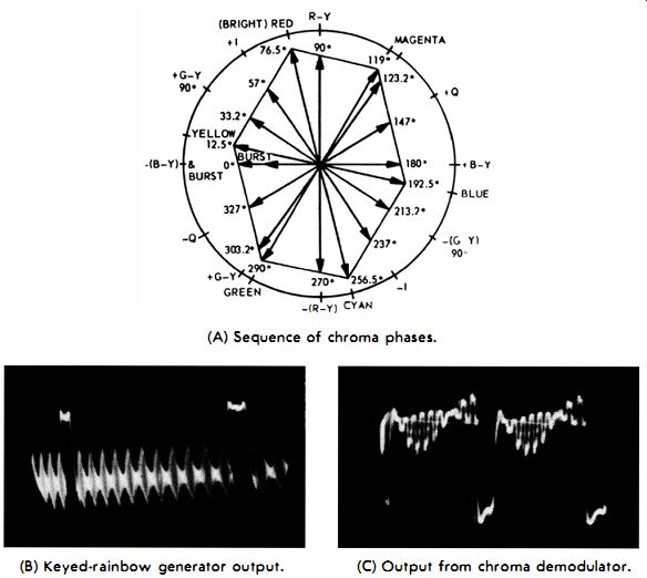
Fig. 6-14. Phase determination with a keyed-rainbow signal. (A) Sequence of chroma phases. (B) Keyed-rainbow generator output. (C) Output from chroma demodulator.

PHASE CHECKS WITH KEYED-RAINBOW SIGNAL

Phase tests and measurements in chroma circuits can also be made with a keyed-rainbow signal. The output from a keyed rainbow generator is illustrated in Fig. 6-14B. Note that 11 "bursts" appear between consecutive horizontal-sync pulses, in 30° intervals. The color burst follows the sync pulse, then G-Y/90° 1 R-Y -(G-Y) Q B-Y -G-Y/90° -I -(R- '" '" " Y) , and G-Y. The -Q phase does not appear in a keyed-rain bow signal, being "lost" on the flyback interval.

When a keyed-rainbow signal is applied to a color receiver and a scope connected at the output of a chroma demodulator, the waveform rises to a maximum and falls to nulls, as illustrated in Fig. 6-14C. The null point (s) is sharply defined, and hence is used to check demodulator phase. Chroma demodulators are quadrature detectors, which means that an R-Y demodulator normally nulls on a B-Y signal, and that a B-Y demodulator nulls on an R-Y signal. A G-Y demodulator normally nulls on a G-Y/90° signal. Similarly, an I demodulator normally nulls on a Q signal, and a Q demodulator nulls on an I signal.

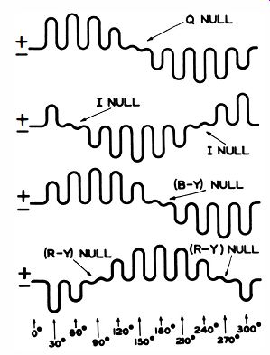
Fig. 6-15. Phase null. for four type. of chroma demodulators. (A) I-demodulator output. (B) Q-demodulator output. (C) (R-Y)-emodulator output. (D) (B-Y)-demodulator output.

Note that the 30° intervals in a keyed-rainbow signal do not all correspond exactly to the various chroma phases. Thus, R-Y and Q are actually 33 ° apart in phase instead of 30°; B-Y and Q are actually 33° apart, instead of 30 degr. However, the 3° phase discrepancy is not serious in practical work, and a keyed-rainbow generator is less costly than an NTSC type generator which is held to close phase tolerances.

Correct phase nulls for four types of chroma demodulators are depicted in Fig. 6-15. A comparison of these waveforms with the diagram in Fig. 6-14A shows that a null normally occurs in a quadrature relation to the reference phase.

Note that a null is obtained from a B-Y demodulator on both R-Y and - (R-Y) phases. Likewise, a null is obtained from a Q demodulator on both I and -I phases. In other words, a phase null is independent of signal polarity. The peak excursions of chroma demodulator waveforms, however, are developed in accordance with signal polarity--thus, an I demodulator output waveform passes first through a positive peak excursion when a rainbow signal is applied, then passes through a null at the Q phase, and then passes through another negative peak excursion. Otherwise stated, the keyed-rainbow signal progresses clockwise in the diagram of Fig. 6-14A, starting at the burst phase and finally returning to the burst phase.