A digital VOM displays a voltage, a current, or a resistance value, not as a quantity indicated by a pointer along a calibrated scale but as an exact or a discrete value. In one example of a digital VOM, shown in Fig. 9-1, there is no judgment factor involved (as there would be with an analog instrument) in deciding that the value displayed is 18.52.
Note, also, that the + sign to the left of the 18.52 indicates that the value is positive. Furthermore, since the FUNCTION switch is set on DC OHMS, and the RANGE switch is set on 20 mA, the value is more specifically understood to be 18.52 mA, dc.
Another example of a digital VOM, or dvm, is the MITS Model DVl600 in Fig. 9-2. It is shown displaying a value of 19.6 volts dc.
Both of the dvm's shown include an automatic-polarity feature, meaning that it is not necessary to be concerned whether or not the common test lead is connected to the negative side and the other test lead to the positive side of the voltage or current source to be measured. The display includes a polarity sign, to indicate whether the "hot" test lead is connected to the negative (- ) or positive (+) side of a circuit. Not all dvm's include this automatic-polarity feature; on some of those that do not, a polarity-reversing switch is provided.
BASIC COMPONENTS OF DIGITAL VOM'S
As shown in Fig. 9-3, the basic components of the digital VOM are a signal-conditioner stage, an analog-to-digital converter (adc ) stage, and a readout or display stage. Each of these stages includes other features which will be discussed later.
Signal Conditioner--At the input, the first stage, which is the signal conditioner, includes a function switch that is set by the user for the type of measurement desired, -dc, +dc, ac, current, or ohms. Also included in the signal-conditioner circuit is a range switch having the same purpose as the range switch in an analog instrument; that is, to reduce the input signal, if necessary, to a value that is within the measurement capability of the next stage (the analog-to-digital converter ). (Typically, the adc has an input limitation of 1 volt. )
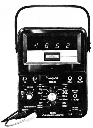
Fig. 9-1. Simpson Model 360 digital VOM.
Some dvm's include "range-changing" circuits. The signal conditioner may also amplify a signal if its level is below that signal level desired. In the signal conditioner, all inputs, whether negative dc voltage, ac voltage, current, or resistance, are converted to positive dc voltages before reaching the adc. Thus, basically, the dvm reads only positive DC voltages.
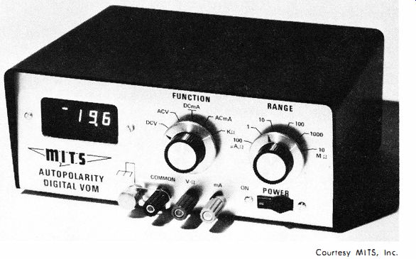
Fig. 9-2. MitS Model DV1600 digital VOM.
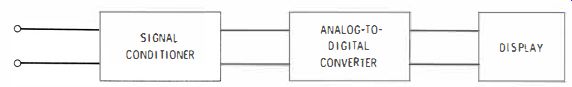
Fig. 9-3 Basic components of a digital VOM.

Fig. 9-4. Arrangement of a 7-segment display as used in a digital voltmeter
readout.
Analog-to-Digital Converter
In the adc, the dc signal being measured is changed from one that may vary continuously over a 0- to 1-volt range to a voltage that varies only in steps or in discrete amounts. Some of the different types of adc's will be discussed later.
Display or Readout
The display or readout is the last basic stage of the dvm. The readout consists of either vacuum-tube, gaseous, or solid-state devices which display a series of self-illuminating numbers between o and 9 to show the numerical value of whatever quantity is being measured. The display device is most often a light-emitting diode (LED), but other types, such as liquid-crystal, incandescent, gas discharge, or Nixie displays, are also used. A minus sign, a plus sign, and/or a decimal point may also be displayed.
Individual numbers in the display are made up of straight-line segments . This means that any number can be produced by lighting the right combination of segments. The arrangement of segments in a 7-segment display is shown in Fig. 9-4. The manner in which different segments are illuminated to produce numbers 0 through 9 is shown in Fig. 9-5.
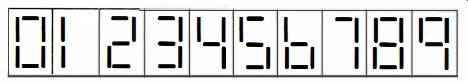
Fig. 9-5. How different segments of a 7-segment display are illuminated to
produce numbers 0 through 9.
TYPES OF ANALOG-TO-DIGITAL CONVERTERS
There are a number of adc circuits, including single linear ramp, dual-slope integration, staircase ramp, and integrating. In all of these, an analog signal is converted to a digital signal. As a simplified example, an analog voltage value is changed into a corresponding interval of time which is used to start and stop an accurately controlled oscillator. The output pulses from the oscillator are fed to a digital counter. The counter has a display that indicates a digital value that is equal to the value of the analog voltage being measured.
The concept of the linear-ramp type of adc is shown in Fig. 9-6.
In this example, the voltage ramp extends from +2 V through 0 to -2 V during an accurately controlled period of time. The voltage to be measured is shown to be 1.8 volts. When the value of the ramp voltage reaches 1.8 volts-that is, when the ramp voltage and the voltage to be measured are equal-a gating pulse is started and an oscillator or clock pulse generator is turned on. The oscillator is turned off when the ramp reaches zero, which is when the gating pulse is turned off. The number of pulses, in this case 10, generated during the gating-pulse time interval, are in direct relation to the voltage to be measured. The pulses are fed to a digital counter readout, which in this example would indicate 1.8 volts.
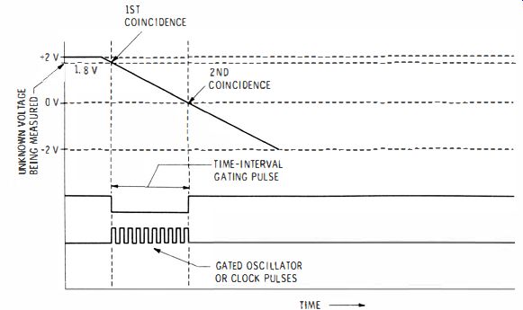
Fig. 9-6. Principle of single-ramp method of analog-to-digital conversion.
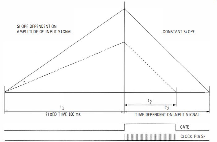
Fig. 9-7. Principle of dual-slope integration method of analog-to-digital
conversion.
The dual-slope, or dual-ramp, adc is perhaps the most widely used. It is a little more complex but somewhat more accurate than the single-ramp method which can be adversely affected by noise.
The principle of the dual-slope, or double-ramp, method of adc, shown in Fig. 9-7, is adapted from the principles of operation of the Philips Model PM2421. The signal to be measured is applied to a capacitor in the input circuit of the instrument. The capacitor is charged by a current proportional to the input signal for a period of 100 milliseconds (ms). The resulting charge is proportional to the mean value of the signal during this interval. At the end of t1 , the charge is then dissipated at a constant-current rate (indicated by "constant slope" in Fig. 9-7 ) for time t2, which will also be proportional to the input signal. Over this period t2, a gate is actuated, providing a series of pulses which are counted and indicated on a digital readout. The readout figure shows the value of the input signal.
In the staircase ramp adc, a sample of the input voltage is compared to an internally generated "staircase ramp" voltage. A block diagram of the Hewlett-Packard Model 3430A digital voltmeter, an instrument employing this method, is shown in Fig. 9-8.
When the input signal, or voltage to be measured, and the staircase ramp voltages are of the same value, the comparator generates a signal to stop the ramp. The instrument readout then displays the number of counts necessary to make the staircase ramp equal to the input voltage. At the end of the sample, a reset pulse from the 2-Hz sample oscillator resets the staircase to zero and the measurement is repeated starting with a new sample. The display shows the value of the previous sample until the next one is completed; the process is repeated every half second.
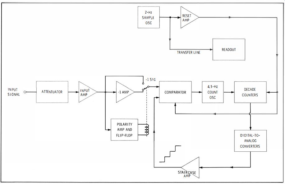
Fig. 9-8
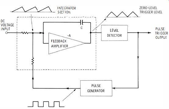
Fig. 9-9. Voltage-to-frequency converter in integrating-type analog-to-digital
converter.
INTEGRATING TYPE OF ANALOG-TO-DIGITAL CONVERTER
In the integrating type of adc, the average of the input voltage is measured over a predetermined measuring period. By use of an integrating circuit at the input, the average value of the voltage to be measured is attained for the measuring interval. Integration allows for relatively accurate measurement of the input voltage even with substantial interference from superimposed noise. The main advantage of this type of converter is its relative immunity to noise interference.
The integrating circuit normally includes an amplifier, designated as -A in Fig. 9-9, as part of the feedback control system in a voltage-to-frequency converter. The feedback control system governs the pulse repetition rate of the pulse generator so that the average voltage of the generated train of rectangular pulses is equal to the DC input voltage. As shown, the level detector regulates the rate or frequency of the pulse generator.
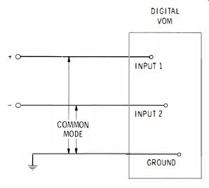
Fig. 9-10. How common-mode interfering signals can enter the input circuit
of a digital VOM.
RESISTANCE MEASUREMENT
In the digital VOM, the resistance-measurement circuit includes a source of constant current which flows through the unknown resistor; then the internal circuitry measures the voltage drop across the resistor and provides a readout of the value of the resistance in ohms.
A particular advantage of the digital VOM is its ability to measure resistance, especially low values, much more accurately than the average analog VOM.
DIGITAL VOLTMETER SPECIFICATIONS
Digital VOM specifications include some that do not apply to, or cannot be interpreted the same way as, those associated with the analog VOM's. These specifications are the accuracy, the resolution, the common-mode rejection, and the normal-mode rejection.
Accuracy--The accuracy of a digital VOM is usually stated in terms of a percentage-of-reading error. There is an additional possible error in the reading of plus-or-minus one digit. For example, a certain digital VOM may have accuracy specified as ±0.75% of full-scale reading, ±1 digit. Thus, for a reading of 130.5 volts on a meter having a 4 digit display, the 0.75% rating would mean that the actual value might be off as much as 130.5 X 0.0075 = 0.98 volt, or approximately 1.0 volt in either the plus or the minus direction. The plus-or-minus-one-digit rating means that the 130.5-volt value could be anywhere between 130.45 and 130.55.
Resolution--The resolution rating of a digital VOM refers to the dynamic range of a VOM. In a 5-digit VOM, the resolution can be 1 part in 100,000 and may be specified as 0.001%. In a 4-digit VOM, the resolution is 1 part in 10,000, or 0.01 %. Common-Mode and Normal-Mode Rejection In digital VOM's having both input terminals isolated from the case of the instrument, an interfering or unwanted signal (say, 60 Hz ) could enter the input circuit through both input terminals with respect to ground, as shown in Fig. 9-10. The ability of a digital VOM to reject such common-mode signals is referred to as its common mode rejection rating and is often specified in decibels.
The ability of a digital VOM to prevent line-frequency interference, noise, and other stray signals from entering the input circuit along with the desired signal is referred to as normal-mode rejection.
DIGITAL VOM RANGES AND "OVERRANGING"
When we change ranges in the analog VOM, we either switch to another scale or use another multiplier, or both. With a digital VOM, there are obviously no scales. Instead, we must observe the location of the decimal point which moves with each different range. We must also be familiar with other digital VOM characteristics referred to as half-digit capability and "over-ranging." For instance, an instrument having 5 digits in the readout display is referred to as a 4 1/2-digit instrument; one having 4 digits is a 3 1/2-digit instrument, and so on. This is because all of the digits except the most significant digit (the one on the left ) can have any value between 0 and 9.
These are referred to as the least Significant digits. The most significant digit can be only 0 or 1; therefore, it is referred to as a "half digit."
The overrange specification for a digital VOM is usually somewhere between 10% and 100%. Overrange may be understood from the following example. In a certain instrument, on the 1000-V setting of the range switch, the left-most digit can go only as high as 1, but all the others can go as high as 9. , Therefore, if the electronic circuitry has been provided in the instrument, the readout can be anything up to 1999 V, or virtually 100% beyond the 1000-V setting of the range switch. Many instruments are provided with 100% overrange capability, but some with 10% only. In the preceding example, a 10% overrange specification would allow an upper-limit reading of only 1100 volts.
If there is an attempt to make a measurement higher than what the instrument is capable of reading at a particular range setting, the usual digital VOM will provide some means to warn the user of the overload. In some instruments, the most significant digit will flash on and off continually; in others a separate overrange warning light comes on.
TYPICAL INSTRUMENTS AND CIRCUITS
In the following pages we will consider a number of typical digital VOMs and discuss their features and circuits. In some cases the features and circuits will be examples of those previously discussed. In other instances, we will be seeing or studying new or improved design features.
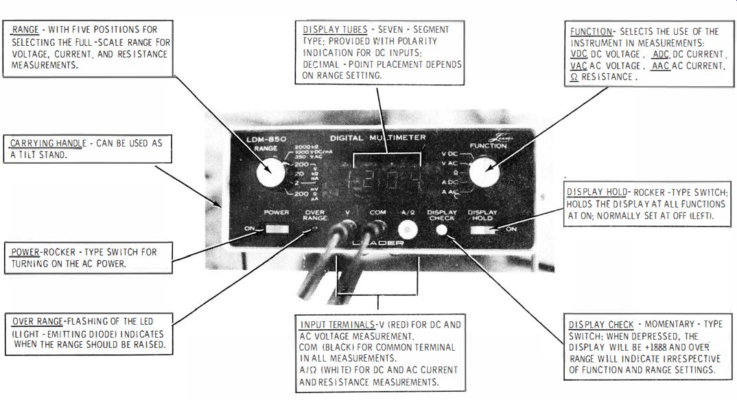
Fig. 9-11 --
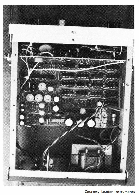
Fig. 9-12. Top view of LDM-850 with cover removed.
Leader Model LDM-8S0 Digital Multimeter
Fig. 9-11 is a front view of the Leader Model LDM-850 digital multimeter, a 3 1/2-digit instrument. Views of the top and bottom, with covers removed, are shown in Figs. 9-12 and 9-13, respectively.
The front view includes identifying the controls and their purposes.
The back of the instrument is provided with legs for vertical operation. Also, on the back panel is a fuse for protection against current or voltage overloads in current- and resistance-measuring circuits.
The ac line cord also exits from the rear panel.
Display Switches
The DISPLAY HOLD switch at the lower right in Fig. 9-11 is normally off, but it may be switched on at any time to hold whatever value is being displayed. The value will then continue to be displayed until the switch is returned to the off position. When the DISPLAY CHECK switch, also at the lower right, is depressed, the display reads +1 8 8 8, which causes all segments in the display tubes to light up. This provides an immediate and continuously available check on the operation of the display section. The decimal point can be checked at each position by moving the Range switch, upper left in Fig. 9-11, through each setting.
The OVERRANGE lamp, lower left of center in Fig. 9-1 1, will light when the value being measured is too high for the range selected; therefore, a higher range must be used. This instrument also includes automatic polarity determination; either a plus or a minus precedes voltage and current readings depending on which side of the circuit being measured is contacted by the red test lead. Also included is an overload protection and an automatic decimal-point placement.
-----------

Chart 9-1. LDM-8S0 Measurement Capabilities
Function Measurement Capabilities
Dc Voltage ±0.1 mV to ±1000 V
Ac Voltage 0. 1 mV to 350 V rms
Resistance 0.1 n to 1999K (1 .999 MO)
Dc Current ±0.1 uA to ±1000 mA
Ac Current 0.1 uA to 1000 mA
-------------
---------
Chart 9-2. Test Current vs Range
Range Max Current RS*
2000K 0.6 uA 10 M-O
200K 6 uA 1M-O
20K 60 uA 100K
2K 60 uA 100K
200 n 600 uA 10K
In series with the internal 6-V source.
---------
Measurement Capabilities
The LDM-850 can measure ac and dc voltage and current as given in Chart 9-1.
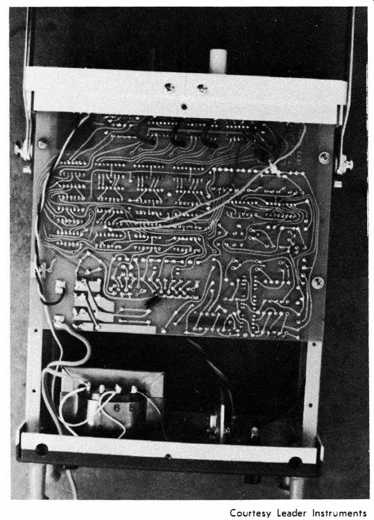
Fig. 9-13. Bottom view of LDM·850 with cover removed.
Resistance Measurements
Using the LDM-850
The following directions for measurement of resistance are taken from the operating manual for the LDM-850. They are fairly typical of those given for most other digital VOM's.
Resistance Measurements--Maximum Resistance: 1999k ohm(1.999M ohm).
1. Connect the black test lead to comterminal and the red test lead to A/D (white ) terminal .
2. Set FUNCTION switch at D. When the test leads are open, there will be an overrange indication.
3. Set RANGE switch at the range under measurement. If the range is not known, set at 200 k-o and lower the range as required.
4. Connect the test lead prods across the resistor or device under test. If the resistor is wired in a circuit, turn off the power be· fore measurement.
5. Read the resistance, k-o, or ohm, referring to the RANGE switch setting.
NOTES:
1. When overrange is indicated during the measurement, lower the range.
2. The figure 00. 1, 00.2, or 00.3 will be displayed when the test leads are shorted at the 200 ohm range.
This represents the resistance of the test leads and terminal contact; it is a normal condition. The value should be subtracted from the displayed value, especially when low resistances are being measured.
3. When measuring resistors wired in a circuit, make certain that there are no other resistors or semiconductors in parallel. Check the schematic.
4. Overload protection (FUNCTION at n): A. 200 n range. The protective fuse will blow if, in error, more than 1 A rms or 1 V rms is applied across the input. B. Other ranges. Will withstand application up to 100 V rms across the input.
Diode and Transistor Checking--Tests for "quality," or forward/ backward resistance characteristic, can be made on diodes and transistors under low current conditions. The procedure is the same as given for resistance measurements.
The maximum currents applicable depend on the RANGE switch settings as given in Chart 9-2.
NOTES : 1. The A/D terminal is the plus (+) side. 2. The forward (or backward) resistance will change at different range settings due to the effect of the internal series resistance, RS. 3. Overload conditions are the same as given for resistance measurements.
Measurement of High Resistances--The procedure for measuring resistance greater than 1999k-o (1.999 M-o ) is given below.
The unknown is connected in parallel with a resistor of known value, 1999kn or less, and the resultant is measured.
The unknown is calculated from the relation : where, Rx = Rstd X R)I k-o Rstd – RM
Rx is the unknown in k-o
Rstd is the known resistance in k ohm R)I is the measured or displayed value in k-o.
For convenience, Rx can be determined with use of the nomogram shown in Fig. 9-14.
In the example, Rstd = 1500k-o, R)I = 1000ko, and Rx = 3000kD (3M-o ).
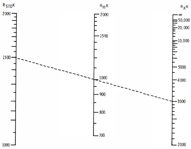
Fig. 9-14. Nomogram for high-resistance measurements (taken from the LDM-850
operating manual).
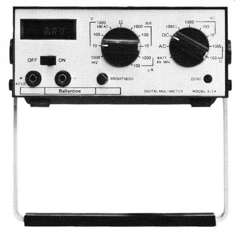
Fig. 9-15. Ballantine Model 3/24 digital multimeter. Courtesy Ballantine laboratories
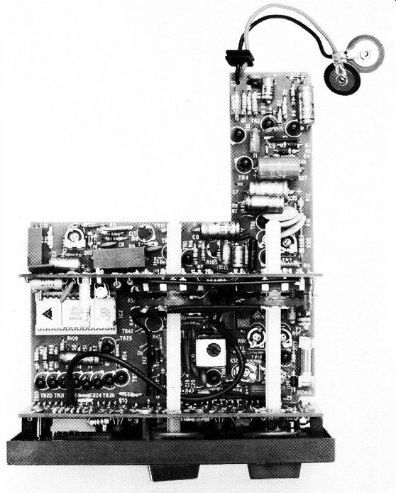
Fig. 9-16. Top view, case removed, of Model 3/24. Courtesy Ballantine Laboratories
Ballantine 3/24 Digital Multimeter The Ballantine Model 3/24 digital multimeter
(shown in Fig. 9 15 ) is a full 3-digit instrument. The "full three digits" means
the maximum reading is 999, rather than 199 as in a 2 1/2-digit instrument.
A top view of the instrument with the case removed is shown in Fig. 9-16. This
instrument is battery operated, but an ac supply is available. When batteries
are used for power, the expected life of the "throw-away" type of
batteries is 300 hours. Power consumption is between 50 and 250 milliwatts
(mW). Battery life is extended by using the BRIGHTNESS control, bottom center
in Fig. 9-15, to reduce the intensity of the LED readout whenever ambient conditions
permit. Automatic polarity is also a feature.
The front panel includes a ZERO screwdriver control (bottom right) to permit exact zero adjustment on all ranges. However, if the ZERO adjustment is used to eliminate the offset of test-lead resistance in the ohmmeter function, the ZERO setting must be returned to normal when the meter is again used for voltage or current measurement.
The normal zero adjustment is accomplished by setting the instrument to the 1000-mV range shorting the test leads together, and adjusting the ZERO control to either 000 or -000. Overloads are indicated by flashing of the most significant digit (which is the left-hand digit ). Some optional accessories are an attenuator probe to minimize loading of the test point and to provide a shielded input lead, an rf probe for extending measurement capability up to 500 MHz for sine-wave signals, and a high-voltage dc probe for extending the normal 1000-V dc maximum capability to 30-kV dc maximum.
The following review of the operation of the display, the analog-to-digital conversion, and the signal-conditioner circuits contains information taken from the instrument service manual.
Display--The three display digits, as shown in Fig. 9-15, are monolithic 7 -segment LEDs. They are time-shared and sequentially switched at a frequency that exceeds the visual flicker rate. Switching is accomplished by a multivibrator in the power supply. The "on" time of each segment can be varied by adjusting the front-panel BRIGHTNESS control which, in turn, adjusts the duty cycle. Movement of the decimal point is accomplished by setting the front-panel RANGE switch.
Analog-to-Digital Conversion--The adc circuit employs a single negative-going ramp generated by a transistor-capacitor combination. The ramp is reset approximately three times per second --actually every 300 milliseconds--and is applied to two comparator amplifiers. One of these provides a reference, and the other provides the unknown dc analog-voltage-input information. The two comparators feed the MOS LSI which also contains the dc auto-polarity indicator circuits. The ramp intercepts generate a time interval which is used in the MOS LSI. A clock oscillator provides a frequency which is counted by the LSI during the measurement time interval.
One thousand counts accumulate during a full-scale measurement.
Display accuracy is maintained through 1200 counts, thus providing 20% overrange.
Signal Conditioners--The signal-conditioner section of Fig. 9-17 includes the input selector switch for voltage, current, and resistance functions, the ac-dc converter, and the dc amp. The ac-to-dc converter is a high-gain differential amplifier which responds to the average value of the incoming ac signal. The instrument actually measures the average value of the input ac but is calibrated in rms volts. The converter is used for both ac voltage and current measurement.
Simpson Model 360 Digital VOM
The Simpson Model 360 digital VOM was shown earlier (Fig. 9-1) in this section, and some of its features were described. Here we will examine the instrument, first as an overall system and then as separate sections (the voltage-, resistance-, and current-measurement circuits; the important power-supply features; and the timing diagram).
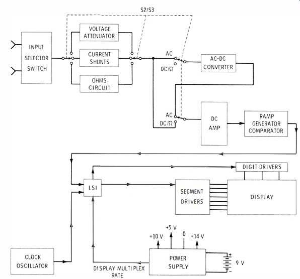
Fig. 9-17. Block diagram of Ballantine 3/24 digital multimeter.
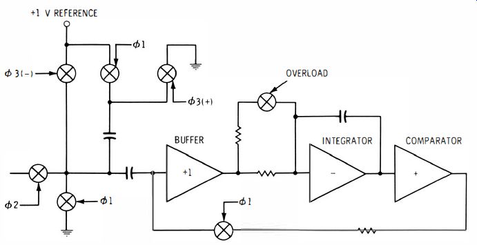
Fig. 9-18. Basic system diagram of the Simpson Model 360 digital VOM.
The Overall System--The simplified basic system diagram for the Simpson 360 digital VOM is shown in Fig. 9-18. The signal or quantity to be measured is connected to the input section consisting of the range, function, and signal-conditioning circuits which convert the input into a proportional and numerically equal dc voltage. The dc voltage is applied to the 3 1/2-digit bipolar or dual-polarity dc digital-voltmeter circuit which is indicated on the digital display, and the analog display, and at the analog output. The analog meter provides for convenient and more-rapid indications for nulling, peaking, and varying signal applications-all of which are a little more difficult to interpret when using a digital readout. The power supply provides ac and dc operating voltages. A choice of battery operation is also available by using rechargeable batteries.
DC Voltage Measurements--The dc voltage being measured is applied to the + and COMMON jacks in Fig. 9-19A and is attenuated, if necessary according to the range selected. This voltage is measured by the digital-voltmeter circuit which provides two basic input sensitivities, 200 m V and 2 V, full range; the two input sensitivities make possible a less-complex attenuator. The same attenuator is used on the 20-V and 200-V ranges, and a separate tap is used for the 1000-V range.
AC Voltage Measurements--The basic circuit for measurement of ac voltage is shown in Fig. 9-19B. The ac voltage being measured is applied to the positive and common jacks and is attenuated, if necessary, by the range switch and then applied to the input amplifier. The amplifier output is converted into dc by the ac-to-dc converter and the dc output is applied to the dc digital voltmeter. The same attenuator and dual-sensitivities system used for dc measurement is also used for ac measurement. The converter responds to the average value of the input signal, but its calibration is based on rms sine-wave value. The operational amplifier includes two rectifying diodes and two feedback resistors, R1 and R2, which drive a summing resistor, R3. The diodes and resistors provide negative feedback to the amplifier input. The rectified signal is filtered and the resulting dc voltage is measured by the dc digital voltmeter circuit which, as already mentioned is calibrated to the rms value of the sine wave being measured.
AC and DC Current Measurements--The ac and dc current-measuring circuits are included in Fig. 9-20. The ac current-measuring circuit is essentially the same as the dc current-measuring circuit, except that for ac measurement the voltage developed across the internal shunt resistance is measured by the ac voltage-measuring circuit.
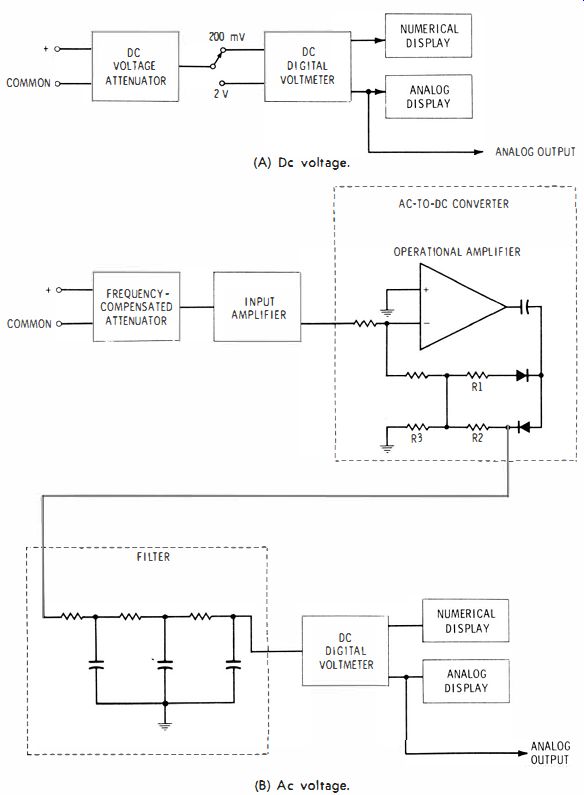
Fig. 9-19. Basic voltage-measurement circuits of the Simpson Model 360. (A)
Dc voltage. (8) Ac voltage.
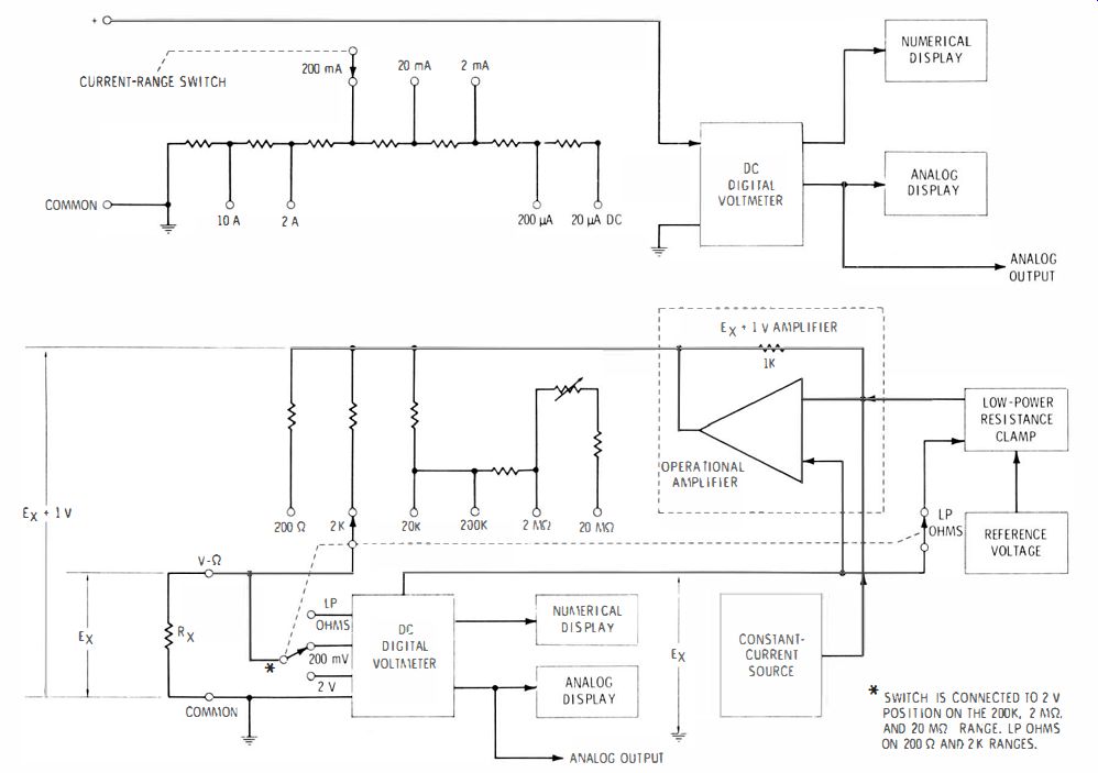
Fig. 9-20.
The basic dc current-measuring circuit is shown in Fig. 9-20A. The dc current being measured is connected in series with the common and the appropriate jack or is connected through the range switch and an internal precision shunt resistance. The shunt resistance used depends on the current range selected so that the voltage across the resistance is proportional and numerically equal to the current through it. This voltage is measured by the digital voltmeter circuit which displays a value equal to the current being measured.
Since the full-range sensitivity of the digital voltmeter circuit is 200 mY, the internal resistance for each current range is equal to 200 m V divided by the full-range current. For example, if the range selected is 200 micro-amperes, the internal resistance selected would be :
200 mV _ 200 x 10-:? _
3.
200 /-LA - 200 x 10-(; - 1 x 10 ,01 1000 ohms
Resistance Measurements--The basic circuit for measurement of resistance in the Simpson Model 360 digital VOM is shown in Fig. 9-20B. Rx represents the resistance to be measured, and it is connected across the V -fl and common jacks. A constant current, generated by the meter, is applied to the unknown resistance, the value of the current being determined by the resistance of the range selected. The current causes a voltage drop across the resistor being measured. This voltage drop is proportional to the value of the unknown resistance. The current through unknown resistance R, is controlled by the operational amplifier which has inputs that "follow" Ex, and the output is always Ex + 1 volt. The current from the constant-current source flows through a 1K feedback resistor and provides the I-volt reference for the amplifier. The (Ex + 1 volt ) output of the amplifier holds the current through Rx at a constant value, regardless of the value of R,. The value of the current is determined by which precision resistor, as selected by the ohms range switch, is in series with R,. The digital voltmeter measures the voltage developed across Rx; the value indicated on the digital readout is equal to the resistance of Rx.
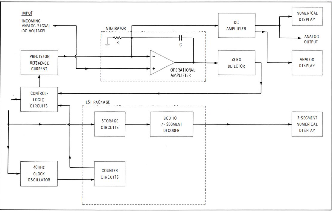
Fig. 9-21
When the digital voltmeter is set for LP OHMS (low-power resistance measurement ), the low-power-resistance clamp limits the voltage across the input terminals to 150 m V, open circuit. Thus, the power applied to R, is limited to less than 100 microwatts. The 200-ohm and 200K settings are the LP OHMS ranges.
Digital Voltmeter Circuit--The digital voltmeter circuit of the Simpson Model 360 VOM is shown in a basic block diagram in Fig. 9-21. The dual-slope integration method of analog-to-digital conversion is used. The incoming dc voltage to be measured is sampled and measured at the integrator input at the rate of approximately 5 times per second. The dc voltage to be measured is sampled during an interval, T1, as indicated in the basic timing diagram (Fig. 9-22 ). The sampling interval is initiated by a pulse from the zero detector circuit, and the measuring interval, T2, is initiated by an "overflow" pulse from the counter circuits. The timing diagram is based on a positive input signal. During interval T1, integrating capacitor C charges and the output voltage from the integrator increases in proportion with the polarity and magnitude of the input signal. At the same time the counter circuits are counting the pulses generated by the 40-kHz clock oscillator. When the count reaches 8000, the counter circuits generate an overflow pulse and the counters reset to the "zero" state.
The overflow pulse gates the control logic circuit which selects a precision current reference of the required polarity and connects it to the integrator input. At this time, the first integrating interval, T1, ends and the second integrating interval, T2, begins. During T2, capacitor C is discharged by the reference current and the voltage at the output of the integrator decreases toward zero. Simultaneously, the counter circuits are counting the 40-kHz clock pulses, continuing until the integrator output becomes zero. At the crossover of zero, the zero detector generates a pulse which, through the control logic circuits, stops the clock oscillator momentarily and transfers the accumulated count to the storage circuits as an equivalent bcd (binary-coded decimal ) signal. The second integrating interval, T2, is now ended; the reference current is disconnected and the cycle repeats, with T1 starting again.
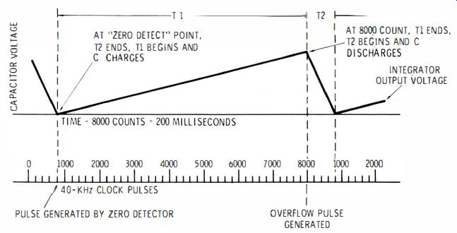
Fig. 9-22. Basic timing diagram of the Simpson 360.
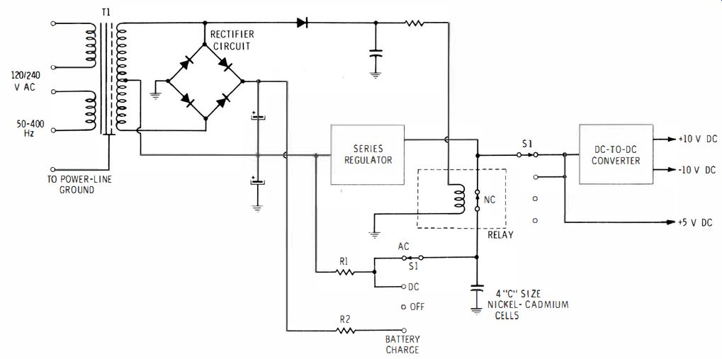
Fig. 9-23
The accumulated bcd signal is converted to signals that the 7 segment decoder/ drivers can use for driving the 7-segment numerical display. The value displayed equals the polarity and numerical value of the analog signal at the integrator input.
Power Supply--The block diagram of the power supply for the Simpson Model 360 VOM is shown in Fig. 9-23. When the VOM is operated from the ac power line, transformer T1 steps down the voltage as required by the rectifier circuit. The rectifier circuit is a full-wave bridge rectifier providing two unregulated dc voltages.
One of the voltages is applied to the series regulator with an output of 5 volts. The R1-R2 network provides battery-charging current when the instrument is operated from a power line. The dc-to-dc converter changes the 5 volts, whether from a regulated power supply or from a battery, into an ac signal which is stepped up and rectified to provide a regulated output of positive 10 volts and negative 10 volts.
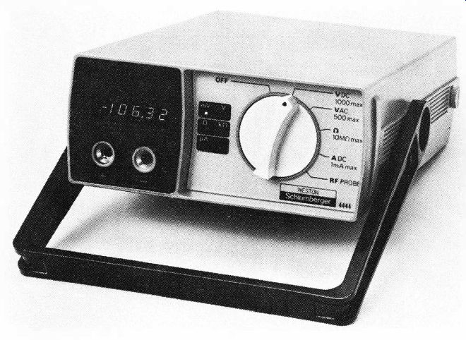
Fig. 9-24. Weston Model 4444 Auto·Ranging digital multimeter. Courtesy Weston
Instruments, Inc.
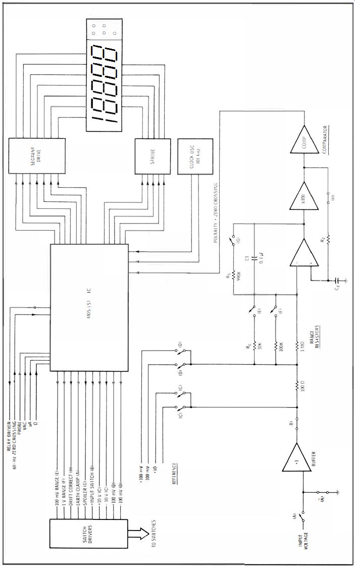
Fig. 9-25. Weston Model 4444 triple-slope converter functional diagram.
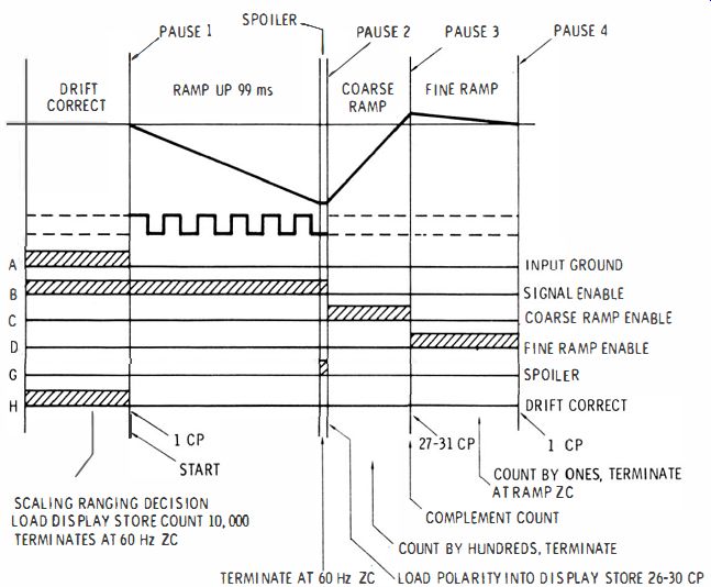
Fig. 9-26. Weston Model 4444 triple-slope converter waveforms.
Weston Model 4444 Auto-Ranging Digital Multimeter
The Weston Model 4444 digital multimeter, shown in Fig. 9-24, includes an automatic-ranging feature, a triple-slope adc, and a 4 ½ digit display.
The theory of operation of the triple-slope conversion process will be explained, according to the manufacturer's service manual, from a functional approach. A complete description of the operating theory, as explained in the manufacturer's instruction manual, is too comprehensive to be included here. The triple-slope converter function diagram is shown in Fig. 9-25, and the waveforms in Fig. 9-26.
The heart of the converter is the integrated circuit, IC, providing all count and control functions. An integrator chain integrates the input voltage and the two reference voltages under control of the IC, and transfers both signal polarity and zero-crossing time to the IC.
A time-shared LED display, shown displaying +18888, is driven automatically by the IC, except for a brief blanking period during the drift-correct period for updating the display store. The master clock for the system is the 101-kHz crystal-controlled 2-phase oscillator. The switches in the integrator chain are either JFETS or MOSFETS driven by driver circuits which are not shown in Fig. 9-25.
Analog-to-Digital Triple-Conversion Cycle--We will now consider the response of the analog-to-digital triple-conversion cycle of the Weston 4444 to a hypothetical input signal of +3.45678 volts; refer to the converter waveforms of Fig. 9-26. We will assume that the 60-Hz power-line waveform is crossing the zero-reference waveform going negative, but that the conversion cycle is continuous and repetitive. The successive steps are as follows:
1. Pause 1--One clock pulse in duration. This delay is required for proper internal function of the IC. A is open; and B is closed, applying zero to the integrator.
2. Ramp Up--10,000 clock pulses (99 milliseconds ) long. During this interval A and B are closed, A open, applying the input signal and causing the integrator to ramp down. Switches E and F, which control sensitivity, are assumed open so that the ramp rate is about (3.5 V /1 Mil X 0.1 uF ) = 35 volts/ second.
The integrator will reach about -3.5 volts in 99 milliseconds.
3. Spoiler--During this interval, switch G closes so that although the input is still applied, the integrator's fall is halted. (The purpose of this step is to improve normal-mode rejection and will be analyzed more fully under Spoiler Operation ). Inputs remain connected through switches A and B until the next negative zero crossing of the power line which initiates Step 4.
4. Pause 2--This lasts between 26 and 30 clock pulses, during which the input signal is grounded and the integrator output remains steady. The polarity of the integrator output and hence of the signal is detected by IC during this interval to determine which reference voltages will be subsequently applied, and to store polarity information for subsequent transfer to the display.
5. Coarse Ramp--During "Coarse Ramp," switches A and B are open, and A and C are closed applying a -10-volt reference.
The integrator ramps back toward zero at 100 volts/second.
The counter chain in the IC will have started at a count of zero and will count each clock pulse as 100 counts during this step.
Since the voltage is 3.45678 volts, it takes between 3456 and 3457 clock pulses to cross zero, an event which is detected by the comparator and passed onto the IC. The ramp will continue until the first clock pulse after zero crossing. The ramp is then terminated by opening switch C. The count remaining on the IC at this time will be 345700 since the system has been counting by hundreds. The overshoot beyond 345678 is 22 counts, which must be subtracted to produce the desired count.
6. Pause 3--This lasts from 27 to 31 clock pulses and serves to complement the count in the 6-decade register with respect to 999999. The complemented count is 654299. Note that subtraction can be achieved by complementing and adding.
7. Fine Ramp--During this step, switch D is closed, applying a + 100-m V reference. The integrator ramps back to zero at 1 volt/ second. Since the integrator had overshot zero for 22 microseconds at 100 volts/ second, a residue of +2.2 millivolt remains. At the new discharge rate of 1 volt/ second, the integrator takes 2.2 milliseconds to reach zero, during which 22 clock pulses are counted. The count is thus brought to 654321 which is internally re-complemented to yield 345678.
8. Pause 4--One clock pulse long-no inputs applied.
9. Drift Correct Period--This final phase has several purposes.
First, the final 6-digit stored number is examined and the four most significant figures are transferred to a display store. In this case, the display would read 3456. In the event of a final count 003456, the same four digits would be transferred but decimal-point position and annunciation would be altered to provide a display of 34.56 mV instead of 3.456 V. (If a number greater than 10999 had been reached, transfer to display would be inhibited and the previous display would continue.) The six-digit number is also examined to determine if a range change is required. If so, switches E or F or the relay are engaged to change the sensitivity of the system for the next cycle.
During all of Step 9, the input to the integrator is maintained at zero by closing B and A and by opening A. The effect of any offsets that are present due to the unity-gain buffer or that are intrinsic to the integrating operational amplifier are fed back through closed switch H to set up a corrective bias on capacitor C2. This phase lasts for 10,000 clock pulses in addition to the time taken for scaling and loading the display, thus ensuring adequate time for the corrective bias to be set up on C2. This bias will maintain itself for the remainder of the succeeding cycle and will be refreshed or updated during the next drift-correct period.
Auto-Ranging--Automatic ranging in the Weston Model 4444 Digital Auto-Ranging Multimeter will be discussed next. This feature makes it unnecessary to select ranges; in fact, only a means for selecting a mode of operation is provided. During the drift-correct period, the 6-digit final count is examined to determine if a range change is needed. The examination takes the form of a search for leading zeros, or overflow beyond 10999. For example, the application of 3.45678 volts when the sensitivity is set at 10 volts (R11 = 1 megohm) gives rise to a count of 34567 in the 6-digit register. No change is required since the best dynamic range of the integrator is being used. A sudden change to 345.678 millivolts will result in a 6-digit count of 034567 (or 34.5678 millivolts to a count of 003456 ). This presence of one Or two leading zeros causes a shift of one or two places to the left before the zero ( s) enters the display store so that only significant data is shown. At the same time, switches F or E, respectively, are closed so that the subsequent conversion will make use of the full dynamic range of the integrator.
Because the interim counts were obtained at an inadequate dynamic range, the last 1 or 2 digits may be in error. However, the reading is transient and recovers to rated accuracy in succeeding conversion cycles. In the interim, a useful display is obtained and the user is not disturbed by the extended inhibit or blanking operation which is characteristic of auto-ranging circuits of earlier design.
If an input larger than 1099 m V but less than 11 volts is applied while the converter is set to maximum sensitivity-Le., 100 m V (Rill = 10K-the converter will inhibit one data transfer and will transfer up range to the 10-volt range after which it will display the data. It will either remain at the 10-volt range or go down range once more to the 1-volt range, depending on the actual level. If an input above 11 volts is suddenly applied, the converter will move up range to 10 volts and then up to 1000 volts, after which it will display and either will remain at 1000 volts or will move down range to 100 volts. No more than 2 conversion intervals can be lost due to ranging.
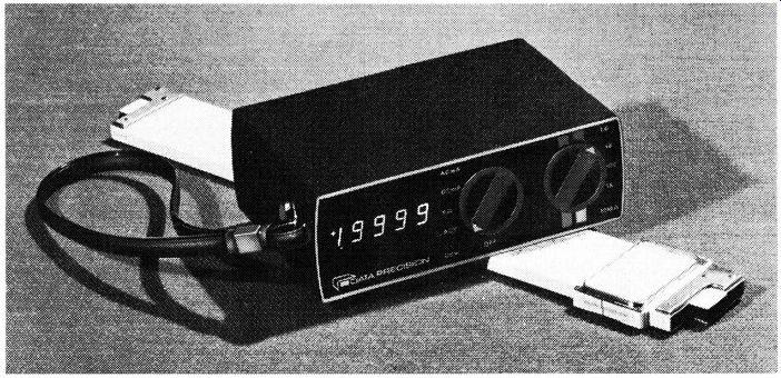
Fig. 9-27. Data Precision Model 245 Tri-Phasic digital voltmeter.
Fig. 9-28. Block diagram of Data Precision Model 245 Tri-Phasic digital voltmeter.
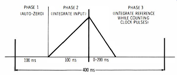
Fig. 9-29. Waveform for the Tri-PhasicTl1 circuit of the Data Precision Model
24S digital voltmeter.
Data-Precision Model 245 Tri-Phasic Digital Multimeter
The Data-Precision Model 245 Tri-Phasic digital multimeter is a 4 1/2-digit instrument. As shown in Fig. 9-27, it is small in size and can be either battery or power-line operated. According to the manufacturer, it is capable of laboratory accuracy. We will consider briefly its Tri-Phasic circuit, which is shown in block-diagram form in Fig. 9-28; its waveform is shown in Fig. 9-29. In the first phase of operation, automatic zero-setting occurs, automatically updating an error integrator/memory circuit, for each conversion cycle. In the second phase, the analog input is integrated together with the stored error, thereby eliminating from the integrated output the offset and drift components that tend to produce errors in certain other digital instruments. The time constant of the integrator is not an accuracy-determining factor. The only accuracy-determining factor is the reference-voltage standard, and the range-divider resistor ratios used only on the higher ranges. In the third phase, the conversion to digital format occurs, returning the integrator to its original zero state, through the original time constant. The Model 245 also includes an Isopolar reference source which provides precise + 1-V and -1-V reference levels through use of one zener diode especially selected for this function. The zener voltage is either reactively or directly coupled to the analog-to-digital converter in a reversible switching arrangement.
Hewlett-Packard Model 970A Digital Multimeter
The Hewlett-Packard Model 970A digital multimeter, shown in Fig. 9-30 is a portable, hand-held, self-contained digital multimeter providing a 3lh-digit readout that can be inverted with the aid of an INVERT DISPLAY switch. The probe tip is built into the end of the instrument. The other test lead is a coiled-pigtail type. A breakdown view of the 970A is shown in Fig. 9-31. Fig. 9-32 shows how convenient it is to use since the instrument can be used in any position and the readout can be inverted, if necessary, by means of the INVERT DISPLAY switch. This instrument features automatic polarity and automatic ranging, ac or DC measurement up to 500 volts, and resistance measurement up to 10 megohms. The test-probe tip is adjustable to several different angles . The analog-to-digital converter of the Hewlett-Packard 970A includes a dual-slope circuit which is generally the same as the circuitry described previously. Referring to the conversion circuit shown in Fig. 9-33 and to the time-interval diagram shown in Fig.9-34, at time t1 the unknown input voltage, Vin, is applied to the integrator. Capacitor C1 then charges at a rate proportional to Vin.
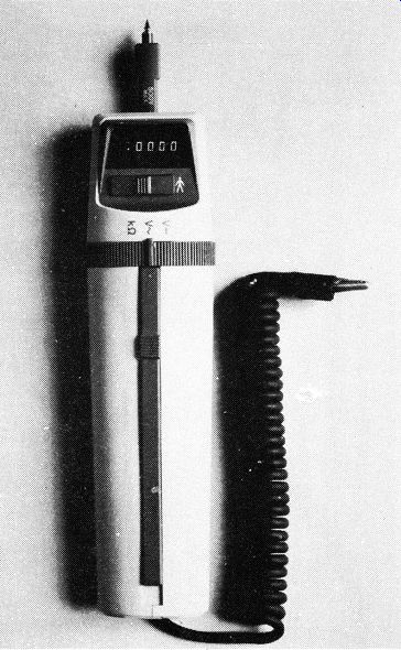
Fig. 9-30. Hewlett-Packard Model 970A. The counter starts totalizing clock
pulses at time t1, and when a predetermined number of clock pulses has been
counted, the control logic switches the integrator input to Vref, a known voltage
with a polarity opposite to that of Vin. This is at time t2• Capacitor C1 now
discharges at a rate determined by V ref.
The counter is reset at time t2, and again it counts clock pulses, continuing to do so until the comparator indicates the integrator output has returned to the starting level, stopping the count. This is at time t3.
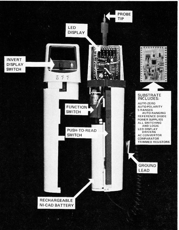
Fig. 9-31. Breakaway view of the Hewlett-Packard Model 970A.
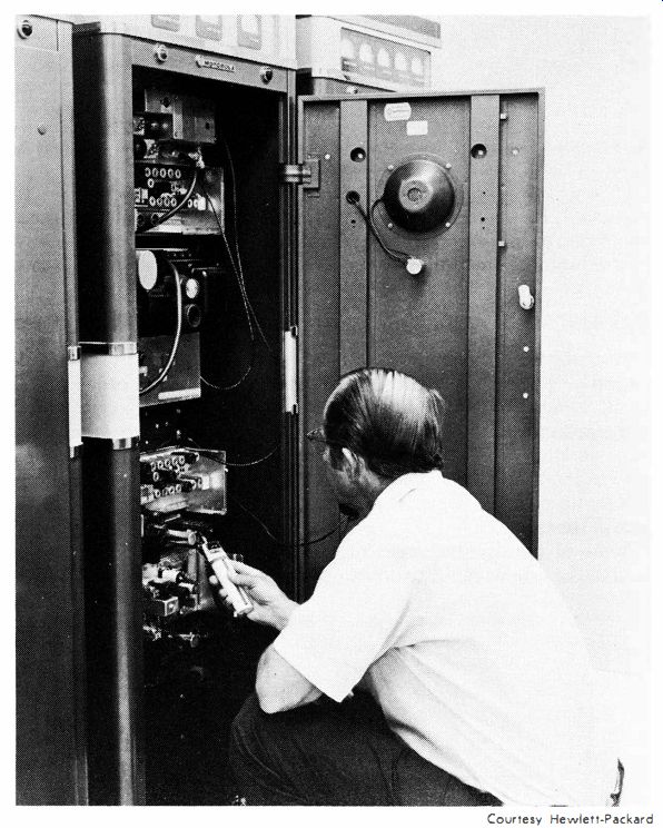
Fig. 9-32. Hewlett-Packard Model 970A being used to make measurements on a
transmitter.
The count retained in the counter is proportional to the input voltage. This is because the time taken for capacitor C1 to discharge is proportional to the charge acquired, which in turn is proportional to the input voltage. The number in the counter is then displayed to give the measurement reading.
The advantage of this technique over the single-slope technique is that many of the variables are self-cancelling. For example, long-term changes in the clock rate or in the characteristics of the integrator amplifier, resistor, or capacitor affect both the charge and the discharge cycles alike. Considerable long-term deviation from normal values can be tolerated without introducing errors . Also, since the input voltage is integrated during the up slope, the final charge on C1 is proportional to the average value of the input during the charge cycle. Noise and other disturbances are thus averaged out and have a reduced effect on the measurement. In particular, by making the charging cycle equal to an integral number of power-line cycles, the effect of any power-line hum is reduced by a substantial amount.
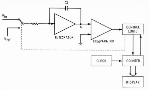
Fig. 9-33. Block diagram of Hewlett-Packard Model 970A analog-to-digital conversion
by the dual-slope technique.
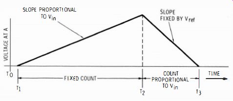
Fig. 9-34. Time-interval diagram for the analog-to-digital conversion in the
Hewlett-Packard 970A.
ADVANTAGES AND DISADVANTAGES OF DIGITAL VOMS
Some of the advantages of digital VOMs have already been discussed or pointed out. A review of some of them is in order at this point. Some of the advantages are: freedom from parallax error, fast and accurate readings, repeatability (different people taking the same reading will come up with the same result ), no eye strain, easy to read, no sticky pointer, automatic ranging and over-ranging, automatic polarity (in most models ), and less skill required on the part of the user.
Some of the disadvantages of digital VOM's are : difficulty in obtaining the rate or rapidity of change in measured values, less rugged and more easily damaged, usually no facility for decibel measurement, less convenient due to usual larger size and need to be operated from a power line (unless battery operated ), difficult to read display under conditions of high surrounding brightness (especially in sunlight ), less useful for semiconductor testing (voltage levels On test leads are not high enough to overcome junction areas, so open-circuit readings are often obtained on good devices ), more expensive than analog instruments, and response to average values of voltage rather than rms values (analog types respond to rms values ).
CARE AND MAINTENANCE OF DIGITAL VOM'S
Reasonable care is required in using all digital VOM's just as in using all analog VOMs. However, there are some special directions which should be followed for specific instruments; these special directions can be obtained from manufacturers' service and operating manuals. These usually include directions for removing and replacing batteries and fuses, doing external and internal cleaning, removing the instrument from the case, testing to ensure proper performance, making zero and calibration checks, and making adjustments. Troubleshooting suggestions are also provided in the usual service manual, plus parts lists and information on obtaining parts or repair service from the manufacturer or from a manufacturer's service center. When you are ordering replacement parts or corresponding with the manufacturer about any instrument, you should provide the following information : instrument model number, serial number, part number, schematic symbol number, identification of part, and description of the problem, if appropriate.
QUESTIONS
1. Name four advantages of digital VOM's over analog types.
2. Name four disadvantages of digital VOM's as compared to analog types.
3. What are the three main stages of a digital VOM?
4. Name 4 types of displays used in digital VOM's.
5. What is the main advantage of the dual-slope analog-to-digital converter as compared to the single-slope type?
6. In which function of a digital VOM is a "constant-current source" employed?
7. How is accuracy usually specified for a digital VOM?
8. If a digital VOM were designed for 20% over-ranging on the 1000-volt range, what is the highest value that could be read on this range?
9. Which digit in a digital display is referred to as the most significant?
10. What would be the purpose of a BRIGHTNESS control on a digital VOM?