by REINHARD METZ
Determine your exposure to line-frequency magnetic-fields with our easy-to-build portable ELF gaussmeter.
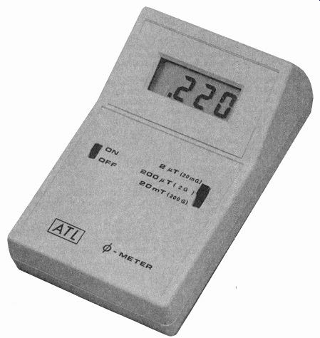
IF YOU ARE ONE IN A GROWING number of people who are concerned about the potentially harmful effects of exposure to magnetic fields, you will be interested in this important construction project. Now you can build your own gaussmeter, and determine the magnitude of magnetic flux densities in and around your home. Our hand held, battery-operated magnetic-field meter is sensitive from 0.1 microtesla (µT) to 20 milliteslas (mT), and has a frequency range from 50 Hz to 20 kHz.
Why all the worry? Magnetic fields are all around us. They occur from the generation, distribution, and use of 50 and 60-Hz electricity, electronic equipment, and even from Earth's magnetic field, which has al ways been present throughout Man's evolution. Man has been "tuned" into Earth's steady magnetic field of about 30 ILT (at sea level) for millions of years. Some sources of excessive magnetic fields that have caused the greatest public concern include power-distribution substations, power lines, CRT terminals, and use of appliances.
Magnetic field intensities can vary greatly, depending on the exposure source and the distance from that source. The rate at which the field intensity falls off with distance can vary from one source to another, depending on how well the current-carrying lines are balanced, or how well the opposing lines of magnetic flux cancel each other out. Fields from coils, magnets, or transformers drop off rapidly with distance by a factor of 1/r3.
In power lines, if currents flow in opposite directions, the drop-off is 1/r2 because of partial field canceling. When unbalanced current exists, the field intensity falls off less rapidly as 1/r.
Figure 1-a, -b, and -c show drop-off rates of 1/r, 142. and 1/r3, respectively. Figure 2 lists some of the many sources of magnetic field exposure, with their range of intensities and drop-off rates.
Although a great deal of controversy still prevails, many people in the scientific community believe that exposure to magnetic fields of extremely-low frequency (ELF fields of 1-100 Hz) may pose a risk to human health. Some disturbing findings of exposure to ELF fields include a significant increase in serum triglycerides (a possible stress indicator) in humans, disorientation of chicks (a result suggesting that bird migration could be affected), and a slowed reaction time in monkeys.
A study conducted by epidemiologist Nancy Wertheimer and physicist Ed Leeper. found that exposures to magnetic fields as small as 0.25 RT correlated with a rise in cancer rates. In the study, the researchers examined wiring and transformers in the neighborhood of birth homes of children who had died of leukemia between 1950 and 1975, along with those of a control group of children who did not have the disease. The results of their studies were published in The American Journal of Epidemiology (March, 1979). Some experts argue that other factors, such as pollution and exposure to chemical carcinogens, make interpretation of those findings very difficult.
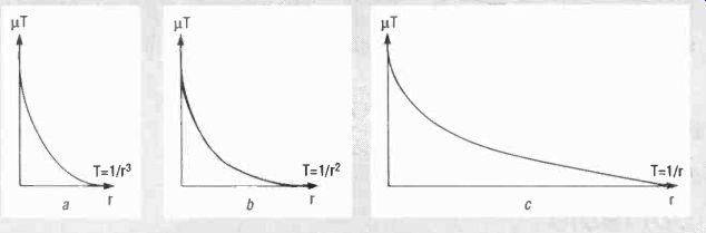
FIG. 1-MAGNETIC FIELD drop-offs. A fast drop-off of 1 r3 (a), 1 r2 (b),
and a slow drop-off of 1/r (c) is typical of many sources of magnetic fields.
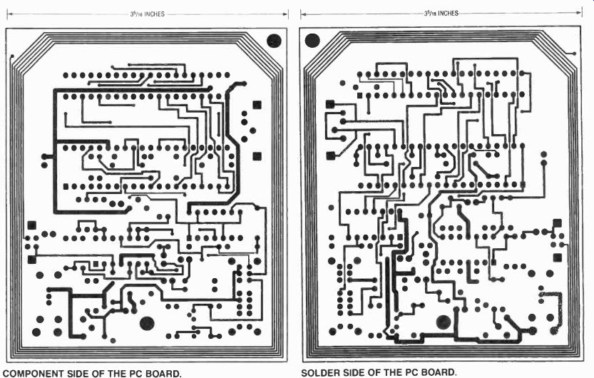
--------- COMPONENT SIDE OF THE PC BOARD. SOLDER SIDE OF THE PC BOARD.
Standards for acceptable exposure to ELF fields are emerging, as are results of studies describing possible hazard levels. If you are more interested a detailed account of scientific findings and the political history of the effects of magnetic-field radiation, we suggest a three-part series of articles by Paul Brodeur, The New Yorker (June 12, 19, and 26, 1989). "60-Hz and The Human Body", IEEE Spectrum, Parts 1-3, Volume 27, Number 9, pages 22-35 (August, 1990) is also a good source for technical information. The Environmental Protection Agency (EPA) has published a report titled "The Evaluation of the Potential Carcinogenicity of Electromagnetic Fields", publication number EPA/600/6-90/005B. This report contains analyses of 64 scientific studies, and is currently under review by the Scientific Advisory Committee.
Well, that's enough back ground for now. Let's examine some of the theory behind how the ELF meter works.
Theory
The quantity of magnetic flux density, B, is in units of webers/ meter2, or tesla (T). The magnetic flux, 4), is defined by the integral 4:1)=.1Bds =B x A where ds is the differential surface area and A is the area that the coil encloses.
For a coil immersed in a field, the induced open-circuit voltage, E, is equal to the number of turns of a coil, N, times the rate of f change of flux through it.
E= IN x dVdtI
Note that the value of N x (14)/dt is actually negative with respect to the induced voltage value, but for our purposes we will just consider the magnitude of the product. The direction of the induced current is such that its own magnetic field opposes the changes in flux responsible for producing it.
If we substitute for 4) we get
E= N x A(dB/dt)
If the magnetic field of a sine wave is B = a(sin tot), a is the amplitude in teslas and 6.) is the angular velocity (230, then dB= aw(cos to Odt. and E= N x Aaw (cos wt)
Since cos wt varies from +1 to-1, the peak magnetic field is defined as E= NAa
For a frequency of 60 Hz, w equals 2n x 60 = 377 For a coil size of 3 1/2" x 3", the area is .0068 m^2, and therefore
E=2.56 Nxa
For the 12-turn pickup coil that we'll use, the sensitivity is 30 µV per µT.
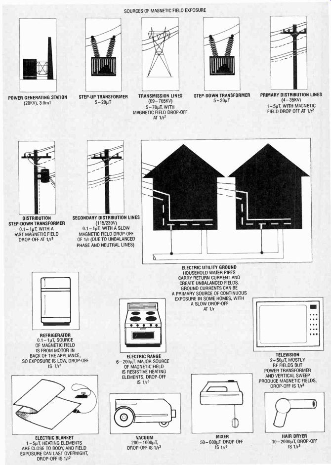
FIG. 2--HERE ARE SOME PRIMARY SOURCES of magnetic field exposure with the
range of field intensity in teslas, and drop-off rates.
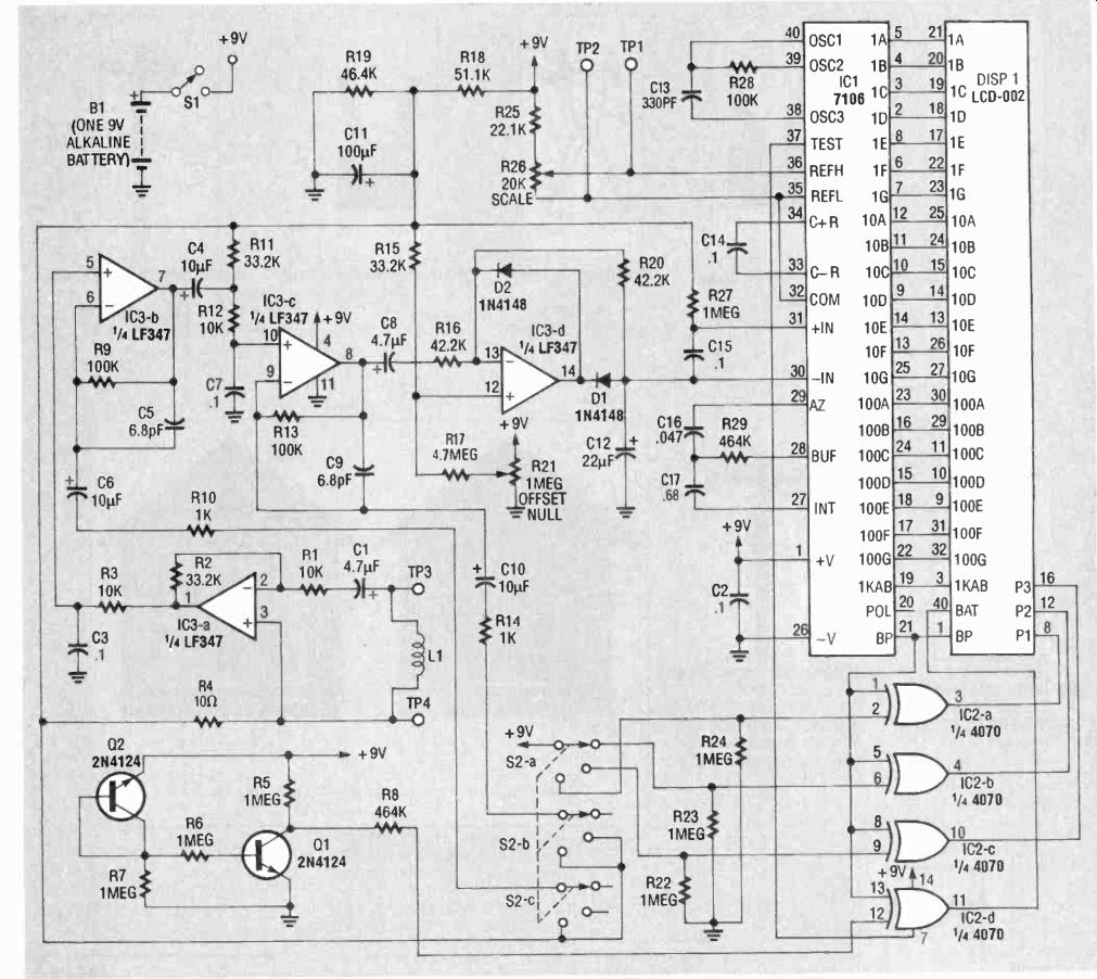
FIG. 3--SCHEMATIC OF THE MAGNETIC FIELD METER. The magnetic field is picked
up by L1 and appears as a voltage that is proportional to the field strength
at the input of IC3 a, which amplifies the signal to 100 µV per µT. The
signal is then further amplified byIC3713 and IC3-c to achieve the three
tesla ranges.
-------------
PARTS LIST
All resistors are 1/4-watt, 1%, unless otherwise indicated.
R1, R3, R12-10,000 ohms
R2, R11, R15-33,200 ohms
R4-10 ohms
R5-R7, R22-R24, R27-1 megohm
R8, R29-464,000 ohms
R9, R13, R28-100,000 ohms
R10, R14-1000 ohms
R16. R20-42,200 ohms
R17-4.7 megohms
R18-51,100 ohms
R19-46,400 ohms
R21-1-megohm potentiometer, 5%
R25-22,100 ohms
R26-20,000-ohm potentiometer, 5%
Capacitors
C1, C8--4.7 µF, 10 volts, electrolytic
C2, C14--0.1 electrolytic or polyester
C3, C7, C15--0.1 µF, polyester
C4, C6, C10--10 µF, electrolytic
C5, C9--6.5 pF, ceramic disc or mica
C11--100 µF, 10 volts, electrolytic
C12-22 10 volts, electrolytic
C13-330 pF, Polyester
C16-0.047 polyester or ceramic disc
C17--0.68 µF, polyester
Semiconductors
D1, D2--1N4148 switching diode
Q1, Q2--2N4124 NPN transistor
IC1-ICL 7106 A/D converter
IC2-4070 or 4030 quad 2-input exclusive-OR gate
IC3-LF347 quad JFET input op–amp
DISP1 LCD-002 liquid crystal display
Other components:
S1-MSS1200, SPST (Alco)
S2-MSS4300. SPDT (Alco)
L1-18 turns, 3" diameter remote-sensing coil (optional, see text)
131-9-volt alkaline battery, with connector Case-Pac-Tec, HPS-9V8
NOTE: The following items are avail able from A & T Labs, P.O. Box 4884, Wheaton, IL 60187: A kit of all parts including PC board and case, with out battery, $79.00; an etched, drilled and plated through PC board with solder mask and silk-screened parts placement, $15.00: a fully assembled and tested unit, $109.00. Add 6.75% sales tax for Illinois residents, 5% shipping and handling in U.S., 12% shipping and handling in Canada.
Check or Money order (UPS COD in contiguous U.S. only) is accepted.
-------------
Circuit description
The meter's 12-turn field pick up is integrated into the unit's circuit board. For remote sensing, an external field coil probe can be used. Figure 3 shows the complete schematic of the circuit. The magnetic field picked up by the coil appears as a voltage, which is proportional to field strength and frequency at the in put of a cascaded amplifier IC3-a, -b, and-c. With a first stage amplifier gain of 3.3 set by R12-R10, the overall sensitivity is 100 µAT per 1.11', or 100 mV per mT. The meter sensitivity is nominally 2 volts full scale, leading to the lowest level sensitivity of 20 mT full scale.
Op-amp IC3-a amplifies the signal to a normalized level of 100 µV per 1 µT. That voltage is further amplified by 1, 100, or 10,000 by IC3-b and-c. The three amplifier stages provide the three magnetic field ranges of 2 mT, 200 µT, and 2 uT (full scale).
Components:
R3-C3 and R12-C7 establish a frequency roll-off characteristic that compensates for the frequency-proportional sensitivity of the pickup coil, and set the 20-kHz cut-off point.
Finally, IC3-d is a precision rectifier and peak detector. Its output drives IC1, a combination analog-to-digital (A/D) converter and LCD driver.
Components
R25-R29 and C13-C17 are used by ICI to set display-update times, clock generation, and reference voltages. The decimal points are driven by IC2, as deter mined by the range-select switch S2.
Transistors
Q1 and Q2 serve as a low-battery detector, and turn on the battery annunciator in the LCD when the battery voltage drops below 7 volts.
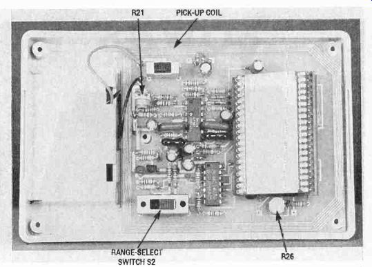
FIG. 4--THIS IS AN INTERNAL VIEW of the magnetic field meter. Assembly
is easy, just install all components below the LCD first.
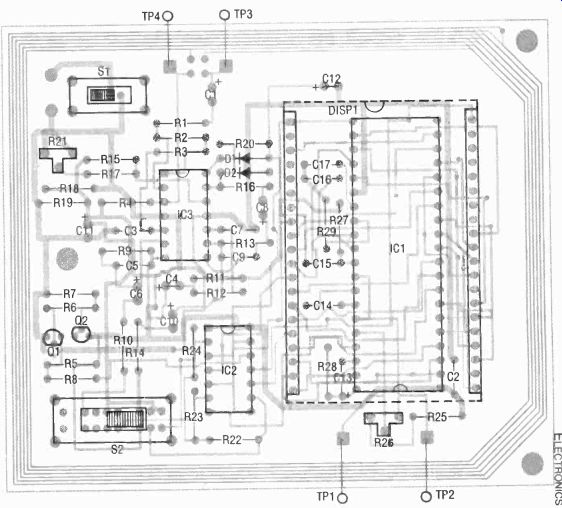
FIG. 5--PARTS PLACEMENT DIAGRAM.
Assembly and checkout
The finished unit shown in Fig. 4 uses a double-sided PC board, which is available from the source mentioned in the parts list. We also show the component side and solder side of the PC board if you choose to make it yourself. You can, however, build the circuit on a perforated construction board if you like, but remember to include the 18-turn remote sensing coil, L1, as indicated in the Parts List. Mount all parts below the LCD display first.
It's easier to fix assembly problems if a socket is used with the LCD. Install all parts as shown in Fig. 5 paying attention to component valves and capacitor polarities. If you are using the internal sensing coil, install jumpers between L1-TP3 and L1-TP4.
If you are using the case specified in the parts list, raise and angle the display as necessary with wire-wrap IC sockets. Make holes in the front panel for Si and S2. Mount the finished PC board in the case using a spacer for the single screw holding the center bottom of the board, and attach the battery connector.
With power on, adjust R26 for 1.000 volt between TP1 and TP2. Then, select the 20 mT range and short the pickup coil with a very short lead between TP3 and TP4.
Adjust offset-null potentiometer R7 for 0.00. Remove the jumper, and the meter is complete.
Calibration
Calibration of the meter is basically determined by the pick up-coil characteristics, amplifier gains, and meter reference-voltage setting. The amplifier gains, as we previously discussed, are chosen to match the coil characteristics as closely as possible.
If you desire to calibrate your meter more exactly, you will need to generate a known magnetic field intensity. One way to do that is to pass a known current through a coil configuration whose field pattern characteristics are known. Figure 6 shows such a calibration setup. A good controllable signal source is a sine-wave generator and an audio amplifier, whose output is coupled to a coil through an 8-ohm resistor. Measuring the voltage across the resistor gives the current. Then, calculate the magnetic field according to Fig. 6.
(Note that while all references to field strength here are made in teslas, gauss are also commonly used. The conversion is easy: 1 tesla = 10,000 gauss.) Place the meter inside the coil and turn it on. Use the highest sensitivity scale that does not overrange the display. An over-range is indicated by a display of 1 followed by three blanks. In most cases, the 2µT range is satisfactory.
Measurement interpretation
A great deal of controversy exists in the emerging understanding of potential health hazards of low-frequency magnetic fields.
The International Radiation Protection Association (IRPA) has set some interim standards based on 1984 World Health Organization guidelines. Those IRPA standards specify a continuous maximum magnetic field exposure for the general public of 100 uT, and 500 uT as the maximum occupational exposure al lowed over the entire working day.

FIG. 6-USE THIS TEST SETUP TO accurately calibrate your meter. A known
current is passed through a coil whose field intensity is known. A sine-wave
generator provides the 60 Hz frequency, and an audio amplifier is coupled
to the coil by an 8-ohm resistor.
Measure the voltage across the resistor, and use the calculations shown.
adapted from: Electronics Now--Electronics Experimenter's Handbook 1996