AMAZON multi-meters discounts AMAZON oscilloscope discounts
Objectives
This Section will help you understand the difference between temperature and heat, the units used for their measurement, thermal time constants, and the most common methods used to measure temperature and heat and their standards.
Topics covered in this Section are as follows:
_ The difference between temperature and heat
_ The various temperature scales
_ Temperature and heat formulas
_ The various mechanisms of heat transfer
_ Specific heat and heat energy
_ Coefficients of linear and volumetric expansion
_ The wide variety of temperature measuring devices
_ Introduction to thermal time constants
1. Introduction
Similar to our every day needs of temperature control for comfort, almost all industrial processes need accurately controlled temperatures. Physical parameters and chemical reactions are temperature dependent, and therefore temperature control is of major importance. Temperature is without doubt the most measured variable, and for accurate temperature control its precise measurement is required. This Section discusses the various temperature scales used, their relation to each other, methods of measuring temperature, and the relationship between temperature and heat.
2. Basic Terms
2.1 Temperature definitions
Temperature is a measure of the thermal energy in a body, which is the relative hotness or coldness of a medium and is normally measured in degrees using one of the following scales; Fahrenheit (F), Celsius or Centigrade (C), Rankine (R), or Kelvin (K).
Absolute zero is the temperature at which all molecular motion ceases or the energy of the molecule is zero.
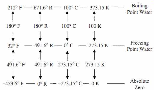
FIG. 1 Comparison of temperature scales.
Fahrenheit scale was the first temperature scale to gain acceptance. It was proposed in the early 1700s by Fahrenheit (Dutch). The two points of reference chosen for 0 and 100° were the freezing point of a concentrated salt solution (at sea level) and the internal temperature of oxen (which was found to be very consistent between animals). This eventually led to the acceptance of 32° and 212° (180° range) as the freezing and boiling point, respectively of pure water at 1 atm (14.7 psi or 101.36 kPa) for the Fahrenheit scale. The temperature of the freezing point and boiling point of water changes with pressure.
Celsius or centigrade scale (C) was proposed in mid 1700s by Celsius (Sweden), who proposed the temperature readings of 0° and 100° (giving a 100° scale) for the freezing and boiling points of pure water at 1 atm.
Rankine scale (R) was proposed in the mid 1800s by Rankine. It is a temperature scale referenced to absolute zero that was based on the Fahrenheit scale, i.e., a change of 1°F = a change of 1°R. The freezing and boiling point of pure water are 491.6°R and 671.6°R, respectively at 1 atm, see FIG. 1.
Kelvin scale (K) named after Lord Kelvin was proposed in the late 1800s. It is referenced to absolute zero but based on the Celsius scale, i.e., a change of 1°C = a change of 1 K. The freezing and boiling point of pure water are 273.15 K and 373.15 K, respectively, at 1 atm, see FIG. 1. The degree symbol can be dropped when using the Kelvin scale.
2.2 Heat definitions
Heat is a form of energy; as energy is supplied to a system the vibration amplitude of its molecules and its temperature increases. The temperature increase is directly proportional to the heat energy in the system.
A British Thermal Unit (BTU or Btu) is defined as the amount of energy required to raise the temperature of 1 lb of pure water by 1°F at 68°F and at atmospheric pressure. It is the most widely used unit for the measurement of heat energy.
A calorie unit (SI) is defined as the amount of energy required to raise the temperature of 1 gm of pure water by 1°C at 4°C and at atmospheric pressure. It is also a widely used unit for the measurement of heat energy.
Joules (SI) are also used to define heat energy and is often used in preference to the calorie, where 1 J (Joule) = 1 W (Watt) × s. This is given in TABLE 1 that gives a list of energy equivalents.
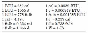
TABLE 1 Conversion Related to Heat Energy
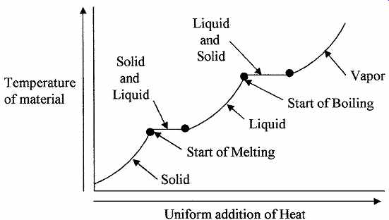
FIG. 2 Showing the relation between temperature and heat energy.
Phase change is the transition of matter from the solid to the liquid to the gaseous states; matter can exist in any of these three states. However, for matter to make the transition from one state up to the next, i.e., solid to liquid to gas, it has to be supplied with energy, or energy removed if the matter is going from gas to liquid to solid. For example, if heat is supplied at a constant rate to ice at 32°F, the ice will start to melt or turn to liquid, but the temperature of the ice liquid mixture will not change until all the ice has melted. Then as more heat is supplied, the temperature will start to rise until the boiling point of the water is reached. The water will turn to steam as more heat is applied but the temperature of the water and steam will remain at the boiling point until all the water has turned to steam, then the temperature of the steam will start to rise above the boiling point. This is illustrated in FIG. 2, where the temperature of a substance is plotted against heat input. Material can also change its volume during the change of phase. Some materials bypass the liquid stage and trans form directly from solid to gas or gas to solid, this transition is called Sublimation.
In a solid, the atoms can vibrate but are strongly bonded to each other so that the atoms or molecules are unable to move from their relative positions. As the temperature is increased, more energy is given to the molecules and their vibration amplitude increases to a point where it can overcome the bonds between the molecules and they can move relative to each other. When this point is reached the material becomes a liquid. The speed at which the molecules move about in the liquid is a measure of their thermal energy. As more energy is imparted to the molecules their velocity in the liquid increases to a point where they can escape the bonding or attraction forces of other molecules in the material and the gaseous state or boiling point is reached.
Specific heat is the quantity of heat energy required to raise the temperature of a given weight of a material by 1°. The most common units are BTUs in the English system, i.e., 1 BTU is the heat required to raise 1 lb of material by 1°F and in the SI system, the calorie is the heat required to raise 1 g of material by 1°C. Thus, if a material has a specific heat of 0.7 cal/g °C, it would require 0.7 cal to raise the temperature of a gram of the material by 1°C or 2.93 J to raise the temperature of the material by 1 k. TABLE 2 gives the specific heat of some common materials; the units are the same in either system.
Thermal conductivity is the flow or transfer of heat from a high temperature region to a low temperature region. There are three basic methods of heat transfer; conduction, convection, and radiation. Although these modes of transfer can be considered separately, in practice two or more of them can be present simultaneously.
2. Specific Heats of Some Common Materials
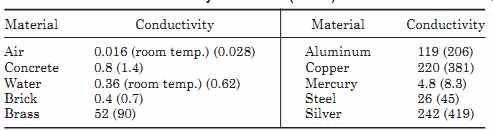
TABLE 3 Thermal Conductivity BTU/h ft °F (W/mK)
Conduction is the flow of heat through a material. The molecular vibration amplitude or energy is transferred from one molecule in a material to the next.
Hence, if one end of a material is at an elevated temperature, heat is conducted to the cooler end. The thermal conductivity of a material k is a measure of its efficiency in transferring heat. The units can be in BTUs per hour per ft per °F or watts per meter-Kelvin (W/m K) (1 BTU/ft h °F = 1.73 W/mK). TABLE 3 gives typical thermal conductivities for some common materials.
Convection is the transfer of heat due to motion of elevated temperature particles in a material (liquid and gases). Typical examples are air conditioning systems, hot water heating systems, and so forth. If the motion is solely due to the lower density of the elevated temperature material, the transfer is called free or natural convection. If the material is moved by blowers or pumps the transfer is called forced convection.
Radiation is the emission of energy by electromagnetic waves that travel at the speed of light through most materials that do not conduct electricity. For instance, radiant heat can be felt some distance from a furnace where there is no conduction or convection.
2.3 Thermal expansion definitions
Linear thermal expansion is the change in dimensions of a material due to temperature changes. The change in dimensions of a material is due to its coefficient of thermal expansion that is expressed as the change in linear dimension (a) per degree temperature change.
Volume thermal expansion is the change in the volume (b) per degree temperature change due to the linear coefficient of expansion. The thermal expansion coefficients for some common materials per degree Fahrenheit are given in TABLE 4. The coefficients can also be expressed as per degree Celsius.
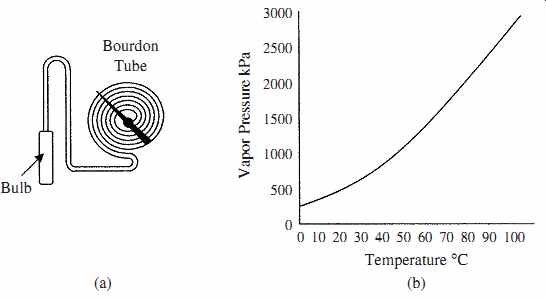
TABLE 4 Thermal Coefficients of Expansion per Degree Fahrenheit
3. Temperature and Heat Formulas
3.1 Temperature
The need to convert from one temperature scale to another is a common every day occurrence. The conversion factors are as follows:
To convert °F to °C
(eqn. 1)
(eqn. 2)
(eqn. 3)
(eqn. 4)
(eqn. 5)
(eqn. 6)
3.2 Heat transfer
The amount of heat needed to raise or lower the temperature of a given weight of a body can be calculated from the following equation:
Q = WC(T2 - T1) (eqn. 7)
where
W = weight of the material
C = specific heat of the material
T2 = final temperature of the material
T1 = initial temperature of the material
Example 2 What is the heat required to raise the temperature of a 1.5 kg mass 120°C if the specific heat of the mass is 0.37 cal/g °C?
Q = 1.5 × 1000 g × 0.37 cal/g °C × 120°C = 66,600 cal
As always, care must be taken in selecting the correct units. Negative answers indicate extraction of heat or heat loss.
Heat conduction through a material is derived from the following relationship:
(eqn. 8)
where
Q = rate of heat transfer
k = thermal conductivity of the material
A = cross-sectional area of the heat flow
T2 = temperature of the material distant from the heat source
T1 = temperature of the material adjacent to heat source
L = length of the path through the material
Note; the negative sign in the Eq. (eqn. 8) indicates a positive heat flow.
Heat convection calculations in practice are not as straight forward as conduction. However, heat convection is given by
Q = hA (T2 - T1) (eqn. 9)
where
Q = convection heat transfer rate
h = coefficient of heat transfer
h = heat transfer area
T2 - T1 = temperature difference between the source and final temperature of the flowing medium
It should be noted that in practice the proper choice for h is difficult because of its dependence on a large number of variables (such as density, viscosity, and specific heat ). Charts are available for h. However, experience is needed in their application.
Heat radiation depends on surface color, texture, shapes involved and the like.
Hence, more information than the basic relationship for the transfer of radiant heat energy given below should be factored in. The radiant heat transfer is given by
(eqn. 10)
where
Q = heat transferred
C = radiation constant (depends on surface color, texture, units used, and the like) A = area of the radiating surface T2 = absolute temperature of the radiating surface T1 = absolute temperature of the receiving surface Example 6 The radiation constant for a furnace is 0.23 × 10⁻⁸ BTU/h ft^2 °F4 , the radiating surface area is 25 ft^2. If the radiating surface temperature is 750°F and the room temperature is 75°F, how much heat is radiated?
3.3 Thermal expansion
Linear expansion of a material is the change in linear dimension due to temperature changes and can be calculated from the following formula:
L2 = L1 [1 + a (T2 - T1)] (eqn. 11)
where L2 = final length
L1 = initial length
a = coefficient of linear thermal expansion
T2 = final temperature
T1 = initial temperature
Volume expansion in a material due to changes in temperature is given by
V2 = V1 [1 + b (T2 - T1)] (eqn. 12)
where
V2 = final volume
V1 = initial volume
b = coefficient of volumetric thermal expansion
T2 = final temperature
T1 = initial temperature
In a gas, the relation between the pressure, volume, and temperature of the gas is given by
(eqn. 13)
where
P1 = initial pressure, V1 = initial volume, T1 = initial absolute temperature, P2 = final pressure, V2 = final volume, T2 = final absolute temperature
4 Temperature Measuring Devices
There are several methods of measuring temperature that can be categorized as follows:
1. Expansion of a material to give visual indication, pressure, or dimensional change
2. Electrical resistance change
3. Semiconductor characteristic change
4. Voltage generated by dissimilar metals
5. Radiated energy
Thermometer is often used as a general term given to devices for measuring temperature. Examples of temperature measuring devices are described below.
4.1 Thermometers
Mercury in glass was by far the most common direct visual reading thermometer (if not the only one). The device consisted of a small bore graduated glass tube with a small bulb containing a reservoir of mercury. The coefficient of expansion of mercury is several times greater than the coefficient of expansion of glass, so that as the temperature increases the mercury rises up the tube giving a relatively low cost and accurate method of measuring temperature. Mercury also has the advantage of not wetting the glass, and hence, cleanly traverses the glass tube without breaking into globules or coating the tube. The operating range of the mercury thermometer is from -30 to 800°F (-35 to 450°C) (freezing point of mercury -38°F [-38°C]). The toxicity of mercury, ease of breakage, the introduction of cost effective, accurate, and easily read digital thermometers has brought about the demise of the mercury thermometer.
Liquids in glass devices operate on the same principle as the mercury thermometer. The liquids used have similar properties to mercury, i.e., high linear coefficient of expansion, clearly visible, non-wetting, but are nontoxic. The liquid in glass thermometers is used to replace the mercury thermometer and to extend its operating range. These thermometers are accurate and with different liquids (each type of liquid has a limited operating range) can have an operating range of from -300 to 600°F (-170 to 330°C).
Bimetallic strip is a type of temperature measuring device that is relatively inaccurate, slow to respond, not normally used in analog applications to give remote indication, and has hysteresis. The bimetallic strip is extensively used in ON/OFF applications not requiring high accuracy, as it is rugged and cost effective. These devices operate on the principle that metals are pliable and different metals have different coefficients of expansion (see TABLE 4). If two strips of dissimilar metals such as brass and invar (copper-nickel alloy) are joined together along their length, they will flex to form an arc as the temperature changes; this is shown in FIG. 3a. Bimetallic strips are usually configured as a spiral or helix for compactness and can then be used with a pointer to make a cheap compact rugged thermometer as shown in FIG. 3b. Their operating range is from -180 to 430°C and can be used in applications from oven thermometers to home and industrial control thermostats.
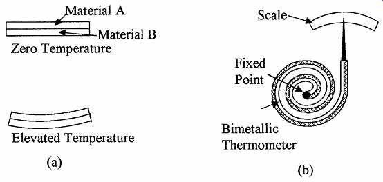
FIG. 3 Shows (a) the effect of temperature change on a bimetallic strip
and (b) bimetallic strip thermometer.
4.2 Pressure-spring thermometers
These thermometers are used where remote indication is required, as opposed to glass and bimetallic devices which give readings at the point of detection. The pressure-spring device has a metal bulb made with a low coefficient of expansion material with a long metal tube, both contain material with a high coefficient of expansion; the bulb is at the monitoring point. The metal tube is terminated with a spiral Bourdon tube pressure gage (scale in degrees) as shown in FIG. 4a. The pressure system can be used to drive a chart recorder, actuator, or a potentiometer wiper to obtain an electrical signal. As the temperature in the bulb increases, the pressure in the system rises, the pressure rise being proportional to the temperature change. The change in pressure is sensed by the Bourdon tube and converted to a temperature scale. These devices can be accurate to 0.5 percent and can be used for remote indication up to 100 m but must be calibrated, as the stem and Bourdon tube are temperature sensitive.
There are three types or classes of pressure-spring devices. These are as follows:
Class 1 Liquid filled
Class 2 Vapor pressure
Class 3 Gas filled
Liquid filled thermometer works on the same principle as the liquid in glass thermometer, but is used to drive a Bourdon tube. The device has good linearity and accuracy and can be used up to 550°C.
FIG. 4 Illustrates (a) pressure filled thermometer and (b) vapor pressure curve for methyl chloride.
Vapor-pressure thermometer system is partially filled with liquid and vapor such as methyl chloride, ethyl alcohol, ether, toluene, and so on. In this system the lowest operating temperature must be above the boiling point of the liquid and the maximum temperature is limited by the critical temperature of the liquid. The response time of the system is slow, being of the order of 20 s. The temperature pressure characteristic of the thermometer is nonlinear as shown in the vapor pressure curve for methyl chloride in FIG. 4b.
Gas thermometer is filled with a gas such as nitrogen at a pressure range of 1000 to 3350 kPa at room temperature. The device obeys the basic gas laws for a constant volume system [Eq.(eqn. 15), V1 = V2] giving a linear relationship between absolute temperature and pressure.
4.3 Resistance temperature devices
Resistance temperature devices (RTD) are either a metal film deposited on a former or are wire-wound resistors. The devices are then sealed in a glass ceramic composite material. The electrical resistance of pure metals is positive, increasing linearly with temperature. TABLE 5 gives the temperature coefficient of resistance of some common metals used in resistance thermometers. These devices are accurate and can be used to measure temperatures from -300 to 1400°F (-170 to 780°C).
In a resistance thermometer the variation of resistance with temperature is given by
RT2 = RT1
(1 + Coeff. [T2 - T1]) (eqn. 14)
where RT2 is the resistance at temperature T2 and RT1 is the resistance at temperature T1.
Example 9 What is the resistance of a platinum resistor at 250°C, if its resistance at 20°C is 1050 ohm
Resistance at 250°C = 1050(1 + 0.00385 [250 - 20])
= 1050(1 + 0.8855)
= 1979.775 ?
Resistance devices are normally measured using a Wheatstone bridge type of system, but are supplied from a constant current source. Care should also be taken to prevent electrical current from heating the device and causing erroneous readings. One method of overcoming this problem is to use a pulse technique. When using this method the current is turned ON for say 10 ms every 10 s, and the sensor resistance is measured during this 10 ms time period. This reduces the internal heating effects by 1000 to 1 or the internal heating error by this factor.
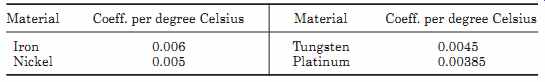
TABLE 5 Temperature Coefficient of Resistance of Some Common Metals
4.4 Thermistors
Thermistors are a class of metal oxide (semiconductor material) which typically have a high negative temperature coefficient of resistance, but can also be positive. Thermistors have high sensitivity which can be up to 10 percent change per degree Celsius, making them the most sensitive temperature elements available, but with very nonlinear characteristics. The typical response times is 0.5 to 5 s with an operating range from -50 to typically 300°C. Devices are available with the temperature range extended to 500°C. Thermistors are low cost and manufactured in a wide range of shapes, sizes, and values. When in use care has to be taken to minimize the effects of internal heating. Thermistor materials have a temperature coefficient of resistance (a) given by
(eqn. 15)
where ?R is the change in resistance due to a temperature change ?T and RS the material resistance at the reference temperature.
The nonlinear characteristics are as shown in FIG. 5 and make the device difficult to use as an accurate measuring device without compensation, but its sensitivity and low cost makes it useful in many applications. The device is normally used in a bridge circuit and padded with a resistor to reduce its nonlinearity.
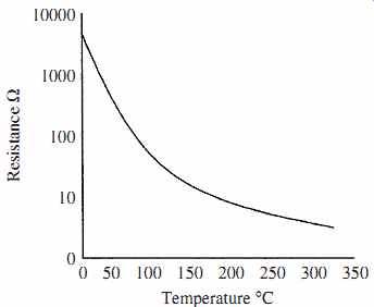
FIG. 5 Thermistor resistance temperature curve.
4.5 Thermocouples
Thermocouples are formed when two dissimilar metals are joined together to form a junction. An electrical circuit is completed by joining the other ends of the dissimilar metals together to form a second junction. A current will flow in the circuit if the two junctions are at different temperatures as shown in FIG. 6a.
FIG. 6 (a) A thermocouple circuit, (b) thermocouples connected to form a thermopile, and (c) focusing EM rays onto a thermopile.
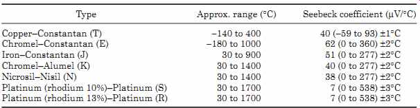
TABLE 6 Operating Ranges for Thermocouples and Seebeck Coefficients
The current flowing is the result of the difference in electromotive force developed at the two junctions due to their temperature difference. In practice, the voltage difference between the two junctions is measured; the difference in the voltage is proportional to the temperature difference between the two junctions. Note that the thermocouple can only be used to measure temperature differences. However, if one junction is held at a reference temperature the voltage between the thermocouples gives a measurement of the temperature of the second junction.
Three effects are associated with thermocouples. They are as follows:
1. Seebeck effect. It states that the voltage produced in a thermocouple is proportional to the temperature between the two junctions.
2. Peltier effect. It states that if a current flows through a thermocouple one junction is heated (puts out energy) and the other junction is cooled (absorbs energy).
3. Thompson effect. It states that when a current flows in a conductor along which there is a temperature difference, heat is produced or absorbed, depending upon the direction of the current and the variation of temperature.
In practice, the Seebeck voltage is the sum of the electromotive forces generated by the Peltier and Thompson effects. There are a number of laws to be observed in thermocouple circuits. Firstly, the law of intermediate temperatures states that the thermoelectric effect depends only on the temperatures of the junctions and is not affected by the temperatures along the leads. Secondly, the law of intermediate metals states that metals other than those making up the thermocouples can be used in the circuit as long as their junctions are at the same temperature, i.e., other types of metals can be used for interconnections and tag strips can be used without adversely affecting the output voltage from the thermocouple. The various types of thermocouples are designated by letters.
Tables of the differential output voltages for different types of thermocouples are available from manufacturer's thermocouple data sheets. TABLE 6 lists some thermocouple materials and their Seebeck coefficient. The operating range of the thermocouple is reduced to the figures in brackets if the given accuracy is required. For operation over the full temperature range the accuracy would be reduced to about ±10 percent without linearization.
Thermopile is a number of thermocouples connected in series, to increase the sensitivity and accuracy by increasing the output voltage when measuring low temperature differences. Each of the reference junctions in the thermopile is returned to a common reference temperature as shown in FIG. 6b.
Radiation can be used to sense temperature. The devices used are pyrometers using thermocouples or color comparison devices.
Pyrometers are devices that measure temperature by sensing the heat radiated from a hot body through a fixed lens that focuses the heat energy on to a thermopile; this is a noncontact device. Furnace temperatures, for instance, are normally measured through a small hole in the furnace wall. The distance from the source to the pyrometer can be fixed and the radiation should fill the field of view of the sensor.
FIG. 6c shows the focusing lens and thermocouple set up in a thermopile.
FIG. 7 shows plots of the electromotive force (emf) versus temperature of some of the types of thermocouples available.
4.6 Semiconductors
Semiconductors have a number of parameters that vary linearly with temperature.
Normally the reference voltage of a zener diode or the junction voltage variations are used for temperature sensing. Semiconductor temperature sensors have a limited operating range from -50 to 150°C but are very linear with accuracies of ±1°C or better. Other advantages are that electronics can be integrated onto the same die as the sensor giving high sensitivity, easy interfacing to control systems, and making different digital output configurations possible. The thermal time constant varies from 1 to 5 s, internal dissipation can also cause up to 0.5°C offset.
Semiconductor devices are also rugged with good longevity and are inexpensive.
For the above reasons the semiconductor sensor is used extensively in many applications including the replacement of the mercury in glass thermometer.
5 Application Considerations
5.1 Selection
In process control a wide selection of temperature sensors are available.
However, the required range, linearity, and accuracy can limit the selection. In the final selection of a sensor, other factors may have to be taken into consideration, such as remote indication, error correction, calibration, vibration sensitivity, size, response time, longevity, maintenance requirements, and cost.
The choice of sensor devices in instrumentation should not be degraded from a cost standpoint. Process control is only as good as the monitoring elements.
5.2 Range and accuracy
TABLE 7 gives the temperature ranges and accuracies of temperature sensors.
The accuracies shown are with minimal calibration or error correction. The ranges in some cases can be extended with the use of new materials. TABLE 8 gives a summary of temperature sensor characteristics.
5.3 Thermal time constant
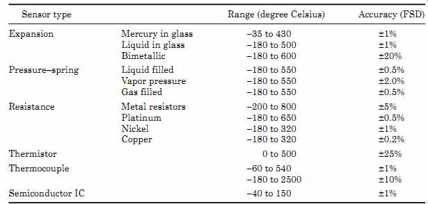
TABLE 7 Temperature Range and Accuracy of Temperature Sensors
A temperature detector does not react immediately to a change in temperature.
The reaction time of the sensor or thermal time constant is a measure of the time it takes for the sensor to stabilize internally to the external temperature change, and is determined by the thermal mass and thermal conduction resistance of the device. Thermometer bulb size, probe size, or protection well can affect the response time of the reading, i.e., a large bulb contains more liquid for better sensitivity, but this will also increase the time constant taking longer to fully respond to a temperature change.
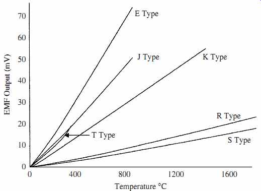
FIG. 7 Thermocouple emf versus temperature for various
types.
The thermal time constant is related to the thermal parameters by the following equation:
(eqn. 16)
where tc = thermal time constant
m = mass
c = specific heat
k = heat transfer coefficient
A = area of thermal contact
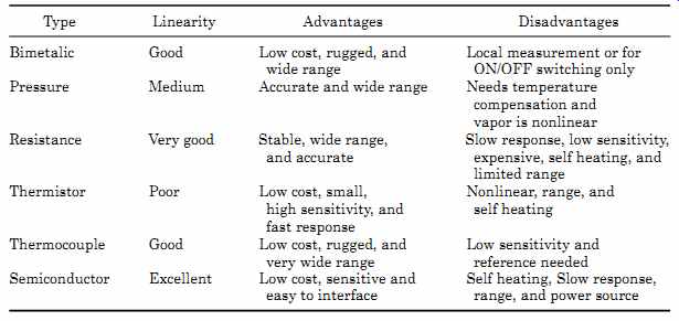
TABLE 8 Summary of Sensor Characteristics
When the temperature changes rapidly, the temperature output reading of a thermal sensor is given by
(eqn. 17)
where T = temperature reading
T1 = initial temperature
T2 = true system temperature
t = time from when the change occurred
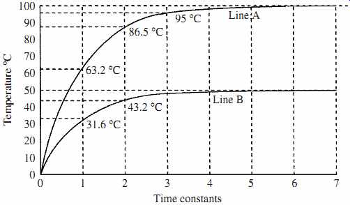
FIG. 8 Shows the response time to changes in temperature.
The time constant of a system tc is considered as the time it takes for the system to reach 63.2 percent of its final temperature value after a temperature change, i.e., a copper block is held in an ice-water bath until its temperature has stabilized at 0°C, it is then removed and placed in a 100°C steam bath, the temperature of the copper block will not immediately go to 100°C, but its temperature will rise on an exponential curve as it absorbs energy from the steam, until after some time period (its time constant) it will reach 63.2°C, aiming to eventually reach 100°C. This is shown in the graph (line A) in FIG. 8. During the second time constant the copper will rise another 63.2 percent of the remaining temperature to get to equilibrium, i.e., (100 - 63.2) 63.2 percent = 23.3°C, or at the end of 2 time constant periods, the temperature of the copper will be 86.5°C. At the end of 3 periods the temperature will be 95° and so on. Also shown in FIG. 8 is a second line B for the copper, the time constants are the same but the final aiming temperature is 50°C. The time to stabilize is the same in both cases. Where a fast response time is required, thermal time constants can be a serious problem as in some cases they can be of several seconds duration. Correction may have to be applied to the output reading electronically to correct for the thermal time constant to obtain a faster response. This can be done by measuring the rate of rise of the temperature indicated by the sensor and extrapolating the actual aiming temperature.
The thermal time constant of a body is similar to an electrical time constant which is discussed in the Section on electricity under electrical time constants.
5.4 Installation
Care must be taken in locating the sensing portion of the temperature sensor, it should be fully encompassed by the medium whose temperature is being measured, and not be in contact with the walls of the container. The sensor should be screened from reflected heat and radiant heat if necessary. The sensor should also be placed downstream from the fluids being mixed, to ensure that the temperature has stabilized, but as close as possible to the point of mixing, to give as fast as possible temperature measurement for good control. A low thermal time constant in the sensor is necessary for a quick response.
Compensation and calibration may be necessary when using pressure-spring devices with long tubes especially when accurate readings are required.
5.5 Calibration
Temperature calibration can be performed on most temperature sensing devices by immersing them in known temperature standards which are the equilibrium points of solid/liquid or liquid/gas mixtures, which is also known as the triple point. Some of these are given in TABLE 9. Most temperature sensing devices are rugged and reliable, but can go out of calibration due to leakage during use or contamination during manufacture and should therefore be checked on a regular basis.
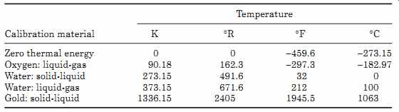
TABLE 9 Temperature Scale Calibration Points
5.6 Protection
In some applications, temperature sensing devices are placed in wells or enclosures to prevent mechanical damage or for ease of replacement. This kind of protection can greatly increase the system response time, which in some circumstances may be unacceptable. Sensors may need also to be protected from over temperature, so that a second more rugged device may be needed to protect the main sensing device. Semiconductor devices may have built in over temperature protection. A fail-safe mechanism may also be incorporated for system shutdown, when processing volatile or corrosive materials.
Summary
This Section introduced the concepts of heat and temperature and their relationship to each other. The various temperature scales in use and the conversion equations between the scales are defined. The equations for heat transfer and heat storage are given. Temperature measuring instruments are described and their characteristics compared.
The highlights of this Section on temperature and heat are as follows:
1. Temperature scales and their relation to each other are defined with examples on how to convert from one scale to the other
2. The transition of material between solid, liquid, and gaseous states or phase changes in materials when heat is supplied
3. The mechanism and equations of heat energy transfer and the effects of heat on the physical properties of materials
4. Definitions of the terms and standards used in temperature and heat measurements, covering both heat flow and capacity
5. The various temperature measuring devices including thermometers, bimetallic elements, pressure-spring devices, RTDs, and thermocouples
6. Considerations when selecting a temperature sensor for an application, thermal time constants, installation, and calibration
Problems
1 Convert the following temperatures to Fahrenheit: 115°C, 456 K, and 423°R.
2 Convert the following temperatures to Rankine: -13°C, 645 K, and -123°F.
3 Convert the following temperatures to Centigrade: 115°F, 356 K, and 533°R.
4 Convert the following temperatures to Kelvin: -215°C, -56°F, and 436°R.
5 How many calories of energy are required to raise the temperature of 3 ft^3 of water 15°F?
6 A 15-lb block of brass with a specific heat of 0.089 is heated to 189°F and then immersed in 5 gal of water at 66°F. What is the final temperature of the brass and water? Assume there is no heat loss.
7 A 4.3-lb copper block is heated by passing a direct current through it. If the voltage across the copper is 50 V and the current is 13.5 A, what will be the increase in the temperature of the copper after 17 min? Assume there is no heat loss.
8 A 129 kg lead block is heated to 176°C from 19°C, how many calories are required?
9 One end of a 9-in long × 7-in diameter copper bar is heated to 59.4°F, the far end of the bar is held at 23°C. If the sides of the bar are covered with thermal insulation, what is the rate of heat transfer?
10 On a winter's day the outside temperature of a 17-in thick concrete wall is -29°F, the wall is 15 ft long and 9 ft high. How many BTUs are required to keep the inside of the wall at 69°? Assume the thermal conductivity of the wall is 0.8 BTU/h ft °F.
11 When the far end of the copper bar in Prob. 9 has a 30-ft^2 cooling fin attached to the end of the bar and is cooled by air convection, the temperature of the f_in rises to t °F. If the temperature of the air is 23°F and the coefficient of heat transfer of the surface is 0.22 BTU/h, what is the value of t?
12 How much heat is lost due to convection in a 25-min period from a 52 ft × 14-ft wall, if the difference between the wall temperature and the air temperature is 54°F and the surface of the wall has a heat transfer ratio of 0.17 BTU/h ft^2 °F?
13 How much heat is radiated from a surface 1.5 ft × 1.9 ft if the surface temperatures is 125°F? The air temperature is 74°F and the radiation constant for the surface is 0.19 × 10^-8 BTU/h ft^2 °F?
14 What is the change in length of a 5-m tin rod if the temperature changes from 11 to 245°C?
15 The length of a 115-ft metal column changes its length to 115 ft 2.5 in when the temperature goes from -40 to 116°F. What is the coefficient of expansion of the metal?
16 A glass block measures 1.3 ft × 2.7 ft × 5.4 ft at 71°F. How much will the volume increase if the block is heated to 563°F?
17 What is the coefficient of resistance per degree Celsius of a material, if the resistance is 2246 ohm at 63°F and 3074 ohm at 405°F?
18 A tungsten filament has a resistance of 1998 ohm at 20°C. What will its resistance be at 263°C?
19 A chromel-alumel thermocouple is placed in a 1773°F furnace. Its reference is 67°F. What is the output voltage from the thermocouple?
20 A pressure-spring thermometer having a time constant of 1.7 s is placed in boiling water (212°F) after being at 69°F. What will be the thermometer reading after 3.4 s?
Related Articles -- Top of Page -- Home