AMAZON multi-meters discounts AMAZON oscilloscope discounts
Objectives
This Section will introduce you to the concepts of fluid velocity and flow and its relation to pressure and viscosity. The Section will help you understand the units used in flow measurement and become familiar with the most commonly used flow standards.
This Section covers the following topics:
_ Reynolds number and its application to flow patterns
_ Formulas used in flow measurements
_ Bernoulli equation and its applications
_ Difference between flow rate and total flow
_ Pressure losses and their effects on flow
_ Flow measurements using differential pressure measuring devices and their characteristics
_ Open channel flow and its measurement
_ Considerations in the use of flow instrumentation
1. Introduction
This Section discusses the basic terms and formulas used in flow measurements and instrumentation. The measurement of fluid flow is very important in industrial applications. Optimum performance of some equipment and operations require specific flow rates. The cost of many liquids and gases are based on the measured flow through a pipeline making it necessary to accurately measure and control the rate of flow for accounting purposes.
2. Basic Terms
This Section will be using terms and definitions from previous Sections as well as introducing a number of new definitions related to flow and flow rate sensing.
Velocity is a measure of speed and direction of an object. When related to fluids it is the rate of flow of fluid particles in a pipe. The speed of particles in a fluid flow varies across the flow, i.e., where the fluid is in contact with the constraining walls (the boundary layer) the velocity of the liquid particles is virtually zero; in the center of the flow the liquid particles will have the maximum velocity. Thus, the average rate of flow is used in flow calculations. The units of flow are normally feet per second (fps), feet per minute (fpm), meters per second (mps), and so on. Previously, the pressures associated with fluid flow were defined as static, impact, or dynamic.
Laminar flow of a liquid occurs when its average velocity is comparatively low and the fluid particles tend to move smoothly in layers, as shown in Fig. 1a.
The velocity of the particles across the liquid takes a parabolic shape.
Turbulent flow occurs when the flow velocity is high and the particles no longer flow smoothly in layers and turbulence or a rolling effect occurs. This is shown in Fig. 1b. Note also the flattening of the velocity profile.
Viscosity is a property of a gas or liquid that is a measure of its resistance to motion or flow. A viscous liquid such as syrup has a much higher viscosity than water and water has a higher viscosity than air. Syrup, because of its high viscosity, flows very slowly and it is very hard to move an object through it. Viscosity (dynamic) can be measured in poise or centipoise, whereas kinematic viscosity (without force) is measured in stokes or centistokes. Dynamic or absolute viscosity is used in the Reynolds and flow equations. TABLE 1 gives a list of con versions. Typically the viscosity of a liquid decreases as temperature increases.
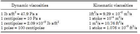
TABLE 1 Conversion Factors for Dynamic and Kinematic Viscosities
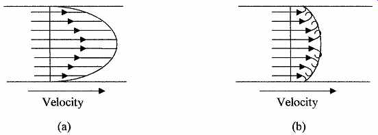
FIG. 1 Flow velocity variations across a pipe with (a) laminar flow
and (b) turbulent flow.
The Reynolds number R is a derived relationship combining the density and viscosity of a liquid with its velocity of flow and the cross-sectional dimensions of the flow and takes the form
(eqn. 1)
where:
V = average fluid velocity
D = diameter of the pipe
r = density of the liquid
m = absolute viscosity
Flow patterns can be considered to be laminar, turbulent, or a combination of both. Osborne Reynolds observed in 1880 that the flow pattern could be predicted from physical properties of the liquid. If the Reynolds number for the flow in a pipe is equal to or less than 2000 the flow will be laminar. From 2000 to about 5000 is the intermediate region where the flow can be laminar, turbulent, or a mixture of both, depending upon other factors. Beyond 5000 the flow is always turbulent.
The Bernoulli equation is an equation for flow based on the law of conservation of energy, which states that the total energy of a fluid or gas at any one point in a flow is equal to the total energy at all other points in the flow.
Energy factors. Most flow equations are based on the law of energy conservation and relate the average fluid or gas velocity, pressure, and the height of fluid above a given reference point. This relationship is given by the Bernoulli equation. The equation can be modified to take into account energy losses due to friction and increase in energy as supplied by pumps.
Energy losses in flowing fluids are caused by friction between the fluid and the containment walls and by fluid impacting an object. In most cases these losses should be taken into account. Whilst these equations apply to both liquids and gases, they are more complicated in gases because of the fact that gases are compressible.
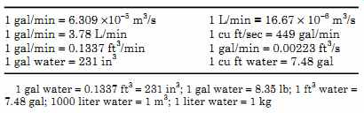
TABLE 2 Flow Rate Conversion Factors
Flow rate is the volume of fluid passing a given point in a given amount of time and is typically measured in gallons per minute (gpm), cubic feet per minute (cfm), liter per minute, and so on. TABLE 2 gives the flow rate con version factors.
Total flow is the volume of liquid flowing over a period of time and is measured in gallons, cubic feet, liters and so forth.
3. Flow Formulas
3.1 Continuity equation
The continuity equation states that if the overall flow rate in a system is not changing with time (see Fig. 2a), the flow rate in any part of the system is constant. From which we get the following equation:
Q = VA (eqn. 2)
where Q = flow rate
V = average velocity
A = cross-sectional area of the pipe
The units on both sides of the equation must be compatible, i.e., English units or metric units.
Example 1 What is the flow rate through a pipe 9 in diameter, if the average velocity is 5 fps?
If liquids are flowing in a tube with different cross section areas, i.e., A1 and A2, as is shown in Fig. 2b, the continuity equation gives:
Q = V1A1 = V2A2 (eqn. 3)
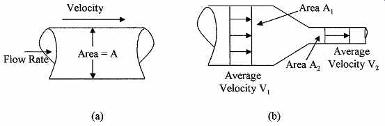
FIG. 2 Flow diagram used for use in the continuity equation: (a) fixed
diameter and (b) effects of different diameters on the flow rate.
3.2 Bernoulli equation
The Bernoulli equation gives the relation between pressure, fluid velocity, and elevation in a flow system. The equation is accredited to Bernoulli (1738). When applied to Fig. 3a the following is obtained-
(eqn. 6)
where PA and PB = absolute static pressures at points A and B, respectively
gA and gB = specific weights
VA and VB = average fluid velocities
g = acc of gravity
ZA and ZB = elevations above a given reference level, i.e., ZA - ZB is the head of fluid.
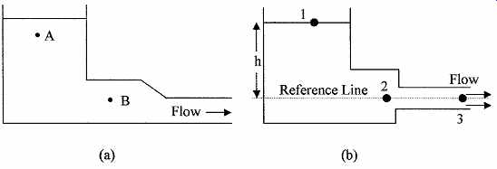
FIG. 3 Container diagrams (a) the pressures at points A and B are related
by the Bernoulli equation and (b) application of the Bernoulli in Example
3.
The units in Eq. (eqn. 6) are consistent and reduce to units of length (feet in the English system and meter in the SI system of units) as follows:
This equation is a conservation of energy equation and assumes no loss of energy between points A and B. The first term represents energy stored due to pressure, the second term represents kinetic energy or energy due to motion, and the third term represents potential energy or energy due to height. This energy relationship can be seen if each term is multiplied by mass per unit volume which cancels as the mass per unit volume is the same at points A and B.
The equation can be used between any two positions in a flow system. The pressures used in the Bernoulli equation must be absolute pressures.
In the fluid system shown in Fig. 3b the flow velocity V at point 3 can be derived from Eq. (eqn. 6) and is as follows using point 2 as the reference line.
(eqn. 7)
Point 3 at the exit has dynamic pressure but no static pressure above 1 atm, and hence, P3 = P1 = 1 atm and g1 = g3. This shows that the velocity of the liquid flowing out of the system is directly proportional to the square root of the height of the liquid above the reference point.
3.3 Flow losses
The Bernoulli equation does not take into account flow losses; these losses are accounted for by pressure losses and fall into two categories. Firstly, those associated with viscosity and the friction between the constriction walls and the flowing fluid, and secondly, those associated with fittings, such as valves, elbows, tees, and so forth.
Outlet losses. The flow rate Q from the continuity equation for point 3 in Fig. 3b for instance gives
Q = V3A3
However, to account for losses at the outlet, the equation should be modified to
Q = CDV3A3 (eqn. 9)
where CD is the discharge coefficient that is dependent on the shape and size of the orifice. The discharge coefficients can be found in flow data handbooks.
Frictional losses. They are losses from liquid flow in a pipe due to friction between the flowing liquid and the restraining walls of the container. These frictional losses are given by:
(eqn. 10)
where:
hL = head loss
f = friction factor
L = length of pipe
D = diameter of pipe
V = average fluid velocity
g = gravitation constant
The friction factor f depends on the Reynolds number for the flow and the roughness of the pipe walls.
To take into account losses due to friction and fittings, the Bernoulli Eq. (eqn. 6) is modified as follows:
(eqn. 12)
Form drag is the impact force exerted on devices protruding into a pipe due to fluid flow. The force depends on the shape of the insert and can be calculated from
(eqn. 13)
where:
F = force on the object
CD = drag coefficient
g = specific weight
g = acceleration due to gravity
A = cross-sectional area of obstruction
V = average fluid velocity
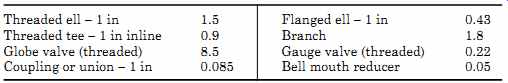
TABLE 3 Typical Head Loss Coefficient Factors for Fittings
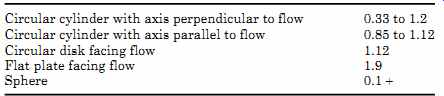
TABLE 4 Typical Drag Coefficient Values for Objects Immersed in Flowing
Fluid
Flow handbooks contain drag coefficients for various objects. TABLE 4 gives some typical drag coefficients.
4. Flow Measurement Instruments
Flow measurements are normally indirect measurements using differential pressures to measure the flow rate. Flow measurements can be divided into the following groups: flow rate, total flow, and mass flow. The choice of the measuring device will depend on the required accuracy and fluid characteristics (gas, liquid, suspended particulates, temperature, viscosity, and so on.)
4.1 Flow rate
Differential pressure measurements can be made for flow rate determination when a fluid flows through a restriction. The restriction produces an increase in pressure which can be directly related to flow rate. FIG. 4 shows examples of commonly used restrictions; (a) orifice plate, (b) Venturi tube, (c) flow nozzle, and (d) Dall tube.
The orifice plate is normally a simple metal diaphragm with a constricting hole. The diaphragm is normally clamped between pipe flanges to give easy access. The differential pressure ports can be located in the flange on either side of the orifice plate as shown in Fig. 4a, or alternatively, at specific locations in the pipe on either side of the flange determined by the flow patterns (named vena contracta). A differential pressure gauge is used to measure the difference in pressure between the two ports; the differential pressure gauge can be calibrated in flow rates. The lagging edge of the hole in the diaphragm is beveled to minimize turbulence. In fluids the hole is normally centered in the diaphragm, see Fig. 5a. However, if the fluid contains particulates, the hole could be placed at the bottom of the pipe to prevent a build up of particulates as in Fig. 5b.
The hole can also be in the form of a semicircle having the same diameter as the pipe and located at the bottom of the pipe as in Fig. 5c.
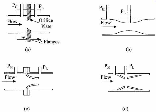
FIG. 4 Types of constrictions used in flow rate measuring devices (a)
orifice plate, (b) Venturi tube, (c) flow nozzle, and (d) Dall tube.
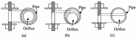
FIG. 5 Orifice shapes and locations used (a) with fluids and (b) and
(c) with suspended solids.
The Venturi tube shown in Fig. 4b uses the same differential pressure principle as the orifice plate. The Venturi tube normally uses a specific reduction in tube size, and is not used in larger diameter pipes where it becomes heavy and excessively long. The advantages of the Venturi tube are its ability to handle large amounts of suspended solids, it creates less turbulence and hence less insertion loss than the orifice plate. The differential pressure taps in the Venturi tube are located at the minimum and maximum pipe diameters. The Venturi tube has good accuracy but has a high cost.
The flow nozzle is a good compromise on the cost and accuracy between the orifice plate and the Venturi tube for clean liquids. It is not normally used with suspended particles. Its main use is the measurement of steam flow. The flow nozzle is shown in Fig. 4c.
The Dall tube shown in Fig. 4d has the lowest insertion loss but is not suit able for use with slurries.
Typical ratios (beta ratios, which are the diameter of the orifice opening divided by the diameter of the pipe) for the size of the constriction to pipe size in flow measurements are normally between 0.2 and 0.6. The ratios are chosen to give high enough pressure drops for accurate flow measurements but are not high enough to give turbulence. A compromise is made between high beta ratios (d/D) which give low differential pressures and low ratios which give high differential pressures, but can create high losses.
To summarize, the orifice is the simplest, cheapest, easiest to replace, least accurate, more subject to damage and erosion, and has the highest loss. The Venturi tube is more difficult to replace, most expensive, most accurate, has high tolerance to damage and erosion, and the lowest losses of all the three tubes. The flow nozzle is intermediate between the other two and offers a good compromise. The Dall tube has the advantage of having the lowest insertion loss but cannot be used with slurries.
The elbow can be used as a differential flow meter. FIG. 6a shows the cross section of an elbow. When a fluid is flowing, there is a differential pressure between the inside and outside of the elbow due to the change in direction of the fluid. The pressure difference is proportional to the flow rate of the fluid.
The elbow meter is good for handling particulates in solution, with good wear and erosion resistance characteristics but has low sensitivity.
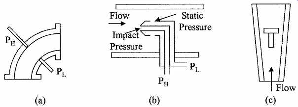
FIG. 6 Other flow measuring devices are (a) elbow, (b) pilot static
tube, and (c) rotameter.
The pilot static tube shown in Fig. 6b is an alternative method of measuring the flow rate, but has some disadvantages in measuring flow, in that it really measures the fluid velocity at the nozzle. Because the velocity varies over the cross section of the pipe, the Pilot static tube should be moved across the pipe to establish an average velocity, or the tube should be calibrated for one area. Other disadvantages are that the tube can become clogged with particulates and the differential pressure between the impact and static pressures for low flow rates may not be enough to give the required accuracy. The differential pressures in any of the above devices can be measured using the pressure measuring sensors discussed in Chap. 5 (Pressure).
Variable-area meters, such as the rotameter shown in Fig. 6c, are often used as a direct visual indicator for flow rate measurements. The rotameter is a vertical tapered tube with a T (or similar) shaped weight. The tube is graduated in flow rate for the characteristics of the gas or liquid flowing up the tube. The velocity of a fluid or gas flowing decreases as it goes higher up the tube, due to the increase in the bore of the tube. Hence, the buoyancy on the weight reduces the higher up the tube it goes. An equilibrium point is eventually reached where the force on the weight due to the flowing fluid is equal to that of the weight, i.e., the higher the flow rate the higher the weight goes up the tube. The position of the weight is also dependent on its size and density, the viscosity and density of the fluid, and the bore and taper of the tube. The Rotameter has a low insertion loss and has a linear relationship to flow rate. In cases where the weight is not visible, i.e., an opaque tube used to reduce corrosion and the like, it can be made of a magnetic material and tracked by a magnetic sensor on the outside of the tube. The rotameter can be used to measure differential pressures across a constriction or flow in both liquids and gases.
An example of rotating flow rate device is the turbine flow meter, which is shown in Fig. 7a. The turbine rotor is mounted in the center of the pipe and rotates at a speed proportional to the rate of flow of the fluid or gas passing over the blades. The turbine blades are normally made of a magnetic material or ferrite particles in plastic so that they are unaffected by corrosive liquids. As the blades rotate they can be sensed by a Hall device or magneto resistive element (MRE) sensor attached to the pipe. The turbine should be only used with clean fluids such as gasoline. The rotating flow devices are accurate with good flow operating and temperature ranges, but are more expensive than most of the other devices.
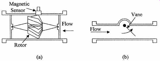
FIG. 7 Flow rate measuring devices (a) turbine and (b) moving vane.
The moving vane is shown in Fig. 7b. This device can be used in a pipe con figuration as shown or used to measure open channel flow. The vane can be spring loaded and able to pivot; by measuring the angle of tilt the flow rate can be determined.
Electromagnetic flow meters can only be used in conductive liquids. The device consists of two electrodes mounted in the liquid on opposite sides of the pipe. A magnetic field is generated across the pipe perpendicular to the electrodes as shown in Fig. 8a. The conducting fluid flowing through the magnetic field generates a voltage between the electrodes, which can be measured to give the rate of flow. The meter gives an accurate linear output voltage with flow rate.
There is no insertion loss and the readings are independent of the fluid characteristics, but it is a relatively expensive instrument.
Vortex flow meters are based on the principle that an obstruction in a fluid or gas flow will cause turbulence or vortices, or in the case of the vortex precession meter (for gases), the obstruction is shaped to give a rotating or swirling motion forming vortices and these can be measured ultrasonically. The frequency of the vortex formation is proportional to the rate of flow and this method is good for high flow rates. At low flow rates the vortex frequency tends to be unstable.
Pressure flow meters use a strain gauge to measure the force on an object placed in a fluid or gas flow. The meter is shown in Fig. 8b. The force on the object is proportional to the rate of flow. The meter is low cost with medium accuracy.
4.2 Total flow
Includes devices used to measure the total quantity of fluid flowing or the volume of liquid in a flow.
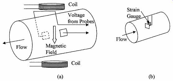
FIG. 8 Flow measuring devices shown are (a) magnetic flow meter and
(b) strain gauge flow meter.
Positive displacement meters use containers of known size, which are filled and emptied for a known number of times in a given time period to give the total flow volume. Two of the more common instruments for measuring total flow are the piston flow meter and the nutating disc flow meter.
Piston meters consist of a piston in a cylinder. Initially the fluid enters on one side of the piston filling the cylinder, at which point the fluid is diverted to the other side of the piston via valves and the outlet port of the full cylinder is opened. The redirection of fluid reverses the direction of the piston and fills the cylinder on the other side of the piston. The number of times the piston traverses the cylinder in a given time frame gives the total flow. The meter has high accuracy but is expensive.
Nutating disc meters are in the form of a disc that oscillates, allowing a known volume of fluid to pass with each oscillation. The meter is illustrated in Fig. 9a. The oscillations can be counted to determine the total volume. This meter can be used to measure slurries but is expensive.
Velocity meters, normally used to measure flow rate, can also be set up to measure the total flow by tracking the velocity and knowing the cross-sectional area of the meter to totalize the flow.
4.3 Mass flow
By measuring the flow and knowing the density of a fluid, the mass of the flow can be measured. Mass flow instruments include constant speed impeller turbine wheel-spring combinations that relate the spring force to mass flow and devices that relate heat transfer to mass flow.
Anemometer is an instrument that can be used to measure gas flow rates. One method is to keep the temperature of a heating element in a gas flow constant and measure the power required. The higher the flow rate, the higher the amount of heat required. The alternative method (hot-wire anemometer) is to measure the incident gas temperature and the temperature of the gas down stream from a heating element; the difference in the two temperatures can be related to the flow rate. Micro-machined anemometers are now widely used in automobiles for the measurement of air intake mass. The advantages of this type of sensor are that they are very small, have no moving parts, pose little obstruction to flow, have a low thermal time constant, and are very cost effective along with good longevity.
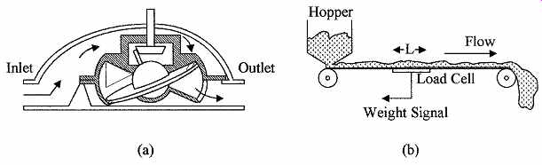
FIG. 9 Illustrations show (a) the cross section of a nutating disc
for the measurement of total flow and (b) conveyer belt system for the measurement
of dry particulate flow rate.
4.4 Dry particulate flow rate
Dry particulate flow rate can be measured as the particulate are being carried on a conveyer belt with the use of a load cell. This method is illustrated in Fig. 9b.
To measure flow rate it is only necessary to measure the weight of material on a fixed length of the conveyer belt.
The flow rate Q is given by
(eqn. 14)
where W = weight of material on length of the weighing platform
L = length of the weighing platform
R = speed of the conveyer belt
Example 7 A conveyer belt is traveling at 19 cm/s, a load cell with a length of 1.1 m is reading 3.7 kgm. What is the flow rate of the material on the belt?
4.5 Open channel flow
Open channel flow occurs when the fluid flowing is not contained as in a pipe but is in an open channel. Flow rates can be measured using constrictions as in contained flows. A weir used for open channel flow is shown in Fig. 10a. This device is similar in operation to an orifice plate. The flow rate is determined by measuring the differential pressures or liquid levels on either side of the constriction. A Parshall flume is shown in Fig. 10b, which is similar in shape to a Venturi tube. A paddle wheel or open flow nozzle are alternative methods of measuring open channel flow rates.
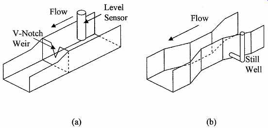
FIG. 10 Open channel flow sensors (a) weir and (b) Parshall flume.
5. Application Considerations
Many different types of sensors can be used for flow measurements. The choice of any particular device for a specific application depends on a number of factors such as- reliability, cost, accuracy, pressure range, temperature, wear and erosion, energy loss, ease of replacement, particulates, viscosity, and so forth.
5.1 Selection
The selection of a flow meter for a specific application to a large extent will depend on the required accuracy and the presence of particulates, although the required accuracy is sometimes down graded because of cost. One of the most accurate meters is the magnetic flow meter which can be accurate to 1 percent of full scale reading or deflection (FSD). The meter is good for low flow rates, with high viscosities and has low energy loss, but is expensive and requires a conductive fluid.
The turbine gives high accuracies and can be used when there is vapor present, but the turbine is better with clean low viscosity fluids. TABLE 5 gives a comparison of flow meter characteristics.
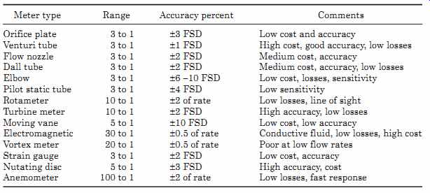
TABLE 5 Summary of Flow Meter Characteristics
The general purpose and most commonly used devices are the pressure differential sensors used with pipe constrictions. These devices will give accuracies in the 3 percent range when used with solid state pressure sensors which convert the readings directly into electrical units or the rotameter for direct visual reading. The Venturi tube has the highest accuracy and least energy loss followed by the flow nozzle and the orifice plate. For cost effectiveness the devices are in the reverse order. If large amounts of particulates are present, the Venture tube is preferred. The differential pressure devices operate best between 30 and 100 per cent of the flow range. The elbow should also be considered in these applications.
Gas flow can be best measured with an anemometer. Solid-state anemometers are now available with good accuracy, are very small in size, and are cost effective.
For open channel applications the flume is the most accurate and best if particulates are present, but is the most expensive.
Particular attention should also be given to manufacturers specifications and application notes.
5.2 Installation
Because of the turbulence generated by any type of obstruction in an otherwise smooth pipe, attention has to be given to the placement of flow sensors. The position of the pressure taps can be critical for accurate measurements. The manufacturer's recommendations should be followed during installation. In differential pressure sensing devices the upstream tap should be one to three pipe diameters from the plate or constriction and the down stream tap up to eight pipe diameters from the constriction.
To minimize the pressure fluctuations at the sensor, it is desirable to have a straight run of 10 to15 pipe diameters on either side of the sensing device. It may also be necessary to incorporate laminar flow planes into the pipe to minimize flow disturbances and dampening devices to reduce flow fluctuations to an absolute minimum.
Flow nozzles may require a vertical installation if gases or particulates are present. To allow gases to pass through the nozzle, it should be facing upwards and for particulates, downwards.
5.3 Calibration
Flow meters need periodic calibration. This can be done by using another calibrated meter as a reference or by using a known flow rate. Accuracy can vary over the range of the instrument and with temperature and specific weight changes in the fluid, which may all have to be taken into account. Thus, the meter should be calibrated over temperature as well as range, so that the appropriate corrections can be made to the readings. A spot check of the readings should be made periodically to check for instrument drift that may be caused by the instrument going out of calibration, particulate build up, or erosion.
Summary
This Section discussed the measurement of the flow of fluids in closed and open channels and gases in closed channels. The basic terms, standards, formulas, and laws associated with flow rates are given. Instruments used in the measurement of flow rates are described, as well as considerations in instrument selection for flow measurement are discussed.
The salient points discussed in this Section are as follows:
1. The relation of the Reynolds number to physical parameters and its use for determining laminar or turbulent flow in fluids
2. The development of the Bernoulli equation from the concept of the conservation of energy, and modification of the equation to allow for losses in liquid flow
3. Definitions of the terms and standards used in the measurement of the flow of liquids and slurries
4. Difference between flow rates, total flow, and mass flow and the instruments used to measure total flow and mass flow in liquids and gases
5. Various types of flow measuring instruments including the use of restrictions and flow meters for direct and indirect flow measurements
6. Open channel flow and devices used to measure open channel flow rates
Comparison of sensor characteristics and considerations in the selection of flow instruments for liquids and slurries and installation precautions
Problems
1 The flow rate in a 7-in diameter pipe is 3.2 ft^3/s. What is the average velocity in the pipe?
2 A 305 liter/min of water flows through a pipe, what is the diameter of the pipe if the velocity of the water in the pipe is 7.3 m/s?
3 A pipe delivers 239 gal of water a minute. If the velocity of the water is 27 ft/s, what is the diameter of the pipe?
4 What is the average velocity in a pipe, if the diameter of the pipe is 0.82 cm and the flow rate is 90 cm3/s?
5 Water flows in a pipe of 23-cm diameter with an average velocity of 0.73 m/s, the diameter of the pipe is reduced, and the average velocity of the water increases to 1.66 m/s. What is the diameter of the smaller pipe? What is the flow rate?
6 The velocity of oil in a supply line changes from 5.1 to 6.3 ft^3/s when going from a large bore to a smaller bore pipe. If the bore of the smaller pipe is 8.1 in diameter, what is the bore of the larger pipe?
7 Water in a 5.5-in diameter pipe has a velocity of 97 gal/s; the pipe splits in two to feed two systems. If after splitting, one pipe is 3.2-in diameter and the other 1.8-in diameter, what is the flow rate from each pipe?
8 What is the maximum allowable velocity of a liquid in a 3.2-in diameter pipe to ensure laminar flow? Assume the kinematic viscosity of the liquid is 1.7 × 10^-5 ft 2/s.
9 A copper sphere is dropped from a building 273 ft tall. What will be its velocity on impact with the ground? Ignore air resistance.
10 Three hundred and eighty five gallons of water per minute is flowing through a 4.3-in radius horizontal pipe. If the bore of the pipe is reduced to 2.7-in radius and the pressure in the smaller pipe is 93 psig, what is the pressure in the larger section of the pipe?
11 Oil with a specific weight of 53 lb/ft^3 is exiting from a pipe whose center line is 17 ft below the surface of the oil. What is the velocity of the oil from the pipe if there is 1.5 ft head loss in the exit pipe?
12 A pump in a fountain pumps 109 gal of water a second through a 6.23-in diameter vertical pipe. How high will the water in the fountain go?
13 What is the head loss in a 7-in diameter pipe 118 ft long that has a friction factor of 0.027 if the average velocity of the liquid flowing in the pipe is 17 ft/s?
14 What is the radius of a pipe, if the head loss is 1.6 ft when a liquid with a friction factor of 0.033 is flowing with an average velocity of 4.3 ft/s through 73 ft of pipe?
15 What is the pressure in a 9.7-in bore horizontal pipe, if the bore of the pipe narrows to 4.1 in downstream where the pressure is 65 psig and 28,200 gal of fluid per hour with a specific gravity (SG) of 0.87 is flowing? Neglect losses.
16 Fluid is flowing through the following 1-in fittings; 3 threaded ells, 6 tees, 7 globe valves, and 9 unions. If the head loss is 7.2 ft, what is the velocity of the liquid?
17 The drag coefficient on a 6.3-in diameter sphere is 0.35. What is its velocity through a liquid with a SG = 0.79 if the drag force is 4.8 lb?
18 A square disc is placed in a moving liquid, the drag force on the disc is 6.3 lbs when the liquid has a velocity of 3.4 ft/s. If the liquid has a density of 78.3 lb/ft 3 and the drag coefficient is 0.41, what is the size of the square?
19 The 8 × 32-in^3 cylinders in a positive displacement meter assembly are rotating at a rate of 570 revolutions an hour. What is the average flow rate per min?
20 Alcohol flows in a horizontal pipe 3.2-in diameter; the diameter of the pipe is reduced to 1.8 in. If the differential pressure between the two sections is 1.28 psi, what is the flow rate through the pipe? Neglect losses.
Related Articles -- Top of Page -- Home