AMAZON multi-meters discounts AMAZON oscilloscope discounts
1. Introduction
This SECTION is designed to introduce the reader to the concept of computer-based data acquisition and to LabVIEW, a software package developed by National Instruments. The main reason for focusing on LabVIEW is its prevalence in laboratory setting. To be sure there are other software tools that support laboratory data acquisition made by a range of vendors. These are reviewed briefly in the appendix due to their limited presence in the educational setting. We should also point out that Matlab and other software tools used to model and simulate dynamic systems are at times used in laboratory setting although their use is often limited to specialized applications such as real-time control. For this reason, these tools are not discussed in this SECTION.
LabVIEW itself is as an extensive programming platform. It includes a multitude of functionalities ranging from basic algebraic operators to advanced signal processing components that can be integrated into rather sophisticated and complex programs. For pedagogical reasons we only introduce the main ideas from LabVIEW that are necessary for functioning in a typical undergraduate engineering laboratory environment. Advanced programming skills can be developed over time as the reader gains comfort with the basic functioning of LabVIEW and its external interfaces.
Specific topics discussed in this SECTION and the associated learning objectives are as follows.
• Structure of personal computer (PC)-based data acquisition (DAQ) systems, the purpose of DAQ cards, and the role of LabVIEW in this context
• Development of simple virtual instruments ( VIs) using basic functionalities of LabVIEW, namely arithmetic and logic operations
• Construction of functionally enhanced VIs using LabVIEW program flow control operations, such as the while loop and the case structure
• Development of VIs that allow for interaction with external hardware as, for instance, acquisition of external signals via DAQ card input channels and generation of functions using DAQ card output channels
These functionalities are essential to using LabVIEW in laboratory setting. Additional capabilities of LabVIEW are explored in the subsequent SECTION on signal processing in LabVIEW.
2. Computer-Based Data Acquisition
In studying mechanical systems, it is often necessary to use electronic sensors to measure certain variables, such as temperature (using thermocouples or RTDs), pressure (using piezoelectric transducers), strain (using strain gauges), and so forth. Although it is possible to use oscilloscopes or multimeters to monitor these variables, it is often preferable to use a PC to view and record the data through the use of a DAQ card. One particular advantage of using computers in this respect is that data can be stored and converted to a format that can be used by spreadsheets (such as Microsoft Excel) or other software packages such as Matlab for more extensive analysis. Another advantage is that significant digital processing of data can be performed in real time via the same platform used to acquire the data. This can significantly improve the process of performing an experiment by making real-time data more useful for further processing.
2.1 Acquisition of Data
One important step in the data acquisition process is the conversion of analogue signals received from sensing instruments to digital representations that can be processed by the computer. Because data must be stored in the computer's memory in the form of individual data points represented by binary numbers, incoming analogue data must be sampled at discrete time intervals and quantized to one of a set of predefined values. In most cases, this is accomplished using a digital-to-analogue (D/A) conversion component on the DAQ card inside the PC or interconnected to it via a Universal Serial Bus (USB) port. Note that both options are used commonly. However, laptop computers and/or low-profile PCs generally require the use of USB-based DAQ devices.
3. National Instruments LabVIEW
LabVIEW is a software package that provides the functional tools and a user interface for data acquisition. Figure 1 depicts a schematic of data flow in the data acquisition process. Note that the physical system may be a mechanical system, such as a beam subjected to stress, a chemical process such as a distillation column, a DC motor with both mechanical and electrical components, and so forth. The key issue here is that certain measurements are taken from the given physical system and are acquired and processed by the PC-based data acquisition system.
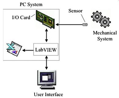
Fig. 1
LabVIEW plays a pivotal role in the data acquisition process. Through the use of VIs, LabVIEW directs the real-time sampling of sensor data through the DAQ card (also known as the I/O card) and is capable of storing, processing, and displaying the collected data. In most cases, one or more sensors transmit analogue readings to the DAQ card in the computer. These analogue data are then converted to individual digital values by the DAQ card and are made available to LabVIEW, at which point they can be displayed to the user. Although LabVIEW is capable of some data analysis functions, it is often preferable to export the data to a spreadsheet for detailed analysis and graphical presentation.
3.1 Virtual Instruments
A VI is a program, created in the LabVIEW programming environment, that simulates physical or hard instruments such as oscilloscopes or function generators. A simple VI used to produce a waveform is depicted in Figure 2. The front panel (shown in Figure 2) acts as the user interface, while data acquisition (in this case the generation process) is performed by a combination of the PC and the DAQ card. Much like the front panel of a real instrument, the front panel window contains controls (i.e., knobs and switches) that allow the user to modify certain parameters during the experiment. These include a selector to choose the type of waveform and numerical controls to choose the frequency and amplitude of the generated waveform, as well as its phase, amplitude and offset.
The front panel of a VI typically also contains indicators that display data or other important information related to the experiment. In this case, a graph is used to depict the waveform. The block diagram(not shown but discussed later) is analogous to the wiring and internal components of a real instrument. The configuration of the VI's block diagram determines how front panel controls and indicators are related. It also incorporates functions such as communicating with the DAQ card and exporting data to disk files in spreadsheet format.
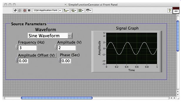
Figure 2
4. Introduction to Graphical Programming in LabVIEW
LabVIEW makes use of a graphical programming language that determines how each VI will work. This section discusses the inner workings of a simple LabVIEW VI used to add and subtract two numbers. While this VI is not particularly useful in a laboratory setting, it illustrates how basic LabVIEW components can be used to construct a VI and hence helps the reader move towards developing more sophisticated VIs. Figure 3 shows the front panel and block diagram of the VI, which accepts two numbers from the user (X and Y) via two simple numeric controls and produces the sum and difference (X ) Y and X + Y) of the numbers displaced on the front panel via two simple numeric indicators.
The block diagram of the VI is a graphical, or more accurately a data flow, program that defines how the controls and indicators on the front panel are interrelated. Controls on the front panel of the VI show values that can be modified by the user while the VI is operating. Indicators display values that are output by the VI. Each control and indicator in the front panel window is associated with a terminal in the block diagram window. Wires in the block diagram window represent the flow of data within the VI. Nodes are additional programming elements that can perform operations on variables, perform input or output functions through the DAQ card, and serve a variety of other functions as well.
The two nodes in the VI shown in Figure 3 (add and subtract) have two inputs and one output, as for instance is depicted in Figure 4. Data can be passed to a node through its input terminals (usually on the left), and the results can be accessed through the node's output terminals, usually on the right.
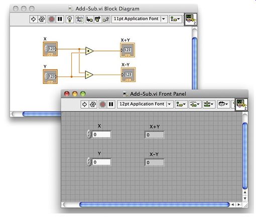
Figure 3
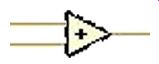
Figure 4
Because LabVIEW diagrams are data flow driven, the sequence in which the various operations in the VI are executed is not determined by the order of a set of commands. Rather, a block diagram node executes when data are present at all of its input terminals. As a result, in the case of the block diagram in Figure 3, one does not know whether the add node or the subtract node will execute first. This issue has implications in more complex applications but is not particularly important in the present context. However, one cannot assume an order of execution merely on the basis of the position of the computational nodes (top to bottom or left to right). If a certain execution order is required or desired, one must explicitly build program flow control mechanisms into the VI, which in practice is not always possible nor is it in the spirit in which LabVIEW was originally designed.
4.1 Elements of the Tools Palette
The mouse pointer can perform a number of different functions in the LabVIEW environment depending on which pointer tool is selected. One can change the mouse pointer tool by selecting the desired tool from the tools palette shown in Figure 5. (If the tools palette does not appear on the screen, it can be displayed by selecting Tools on the View menu.) Choices available in the tools palette are as follows:
• Automatic tool selection. Automatically selects the tool it assumes you need depending on context. For instance, it can be the positioning tool, the wiring tool, or the text tool as further noted later.
• Operating tool. This tool is used operate the front panel controls before or while the VI is running.
• Positioning tool. This tool is used to select, move, or resize objects in either the front panel or the diagram windows. For example, to delete a node in a diagram, one would first select the node with the positioning tool and then press the delete key.
• Text tool. This tool is used to add or change a label. The enter key is used to finalize the task.
• Wiring tool. This tool is used to wire objects together in the diagram window.
When this tool is selected, you can move the mouse pointer over one of a node's input or output terminals to see the description of that terminal.
One can add controls and indicators to the front panel of a VI by dragging and dropping them from the controls palette depicted in Figure 6 and which is visible only when the front panel window is active.
If, for some reason, the controls palette is not visible, one can access it by right clicking anywhere in the front panel window. Once a control or indicator is added to the front panel of a VI, the corresponding terminal is created automatically in the block diagram window.
Adding additional nodes to the block diagram requires use of the functions palette, which is accessible once the block diagram window is visible. One can add arithmetic and logic elements to the block diagram window by dragging and dropping these elements from the functions palette. The functions to add, subtract, and so on can be found in the numeric sub-palette of the programming section of the functions palette (Figure 7, the fourth icon from the left). One can also use constants from the numeric sub-palette in a block diagram and wire those constants as inputs to various nodes.
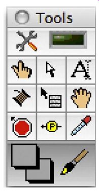
Figure 5
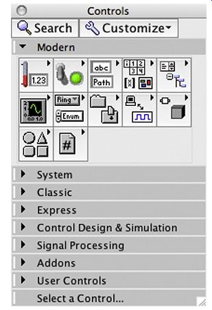
Figure 6
5. Logic Operations in LabVIEW
In more complex VIs, one may encounter situations where the VI must react differently depending on the condition at hand. For example, in a data acquisition process, the VI may need to turn on a warning light when an input voltage exceeds a certain threshold and therefore it may be necessary to compare the input voltage with the threshold value. In addition, the VI needs to make a decision based on the result of the comparison (turn on a light on the screen or external to the DAQ system, produce an alarm sound, etc.). To allow for these types of applications, many logic operators are available in LabVIEW. These can be found in the comparison sub-palette of the programming section of the functions palette. Note that as stated earlier, the functions palette is available when the diagram window is the top (focus) window on the screen.
If one needs to identify the comparison sub-palette, one can move the mouse pointer over the programming section of the palette to call out the different sub-palettes.
Comparison nodes, as, for instance, depicted in Figure 8, are used to compare two numbers.
Their output is either true or false. This value can be used to make decisions between two numbers as shown in Figure 8. Another important node in this respect is the select node, which is also available in the same sub-palette. This node makes a decision based on the outcome of a previous comparison, such as depicted in Figure 8. If the select node's middle input is true, it selects its top input as its output. If its middle input is false, it selects its bottom input as its output. In this way, one can pair the comparison nodes with a select node to produce an appropriate action for subsequent processing.
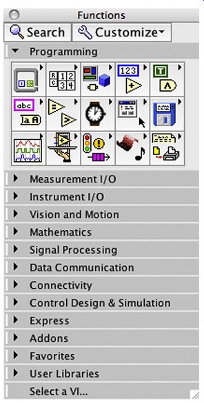
Figure 7
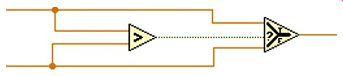
Figure 8
6. Loops in LabVIEW
In building more sophisticated VIs it will not be sufficient to simply perform an operation once.
For example, if LabVIEW is being used to compute the factorial of an integer, n, the program will need to continue to multiply n by n +1, n + 2, and so forth. More pertinently, in data acquisition processes, one needs to acquire multiple samples of data and process the data. For this reason,
LabVIEW includes several types of loop structures. These can be found in the structures subpalette of the programming section in the functions palette. (Note that as with every one of LabVIEW's tools, one can use LabVIEW's help feature or its quick help feature to get more information on these constructs.) Here the user can find a while loop, a for loop, a case statement, and several other important loop structures. Figure 9 depicts a simple program that utilizes a loop.
There are several important items to note about using loops. Everything contained inside the loop will be repeated until the ending condition of the loop is met. For awhile loop, this will be some type of logical condition. In our example given earlier, we have used a button to stop the loop. The loop will stop when a value of true is passed to the stop button at the completion of the loop.
In addition, it is often important to be able to pass values from one iteration to the next. In the example given previously, we needed to take the number from the last iteration and add one to it. This is accomplished using a shift register. To add a shift register, one has to right click (or option click on a Mac) on the right or left side of the loop and use the menu that opens up to add the shift register. To use the shift register, one must wire the value to be passed to the next iteration to the right side as shown in Figure 9. To use the value from the previous iteration, one draws wire from the left side of the loop box to the terminal of one's choosing. In addition, elements initially wired together can be included in a loop simply by creating one around these elements. The wiring initially in place will be preserved. Finally, note that the metronome in the loop times the loop so that it runs every 100ms.This element is available from the timing subpalette in the programming section of the functions palette.
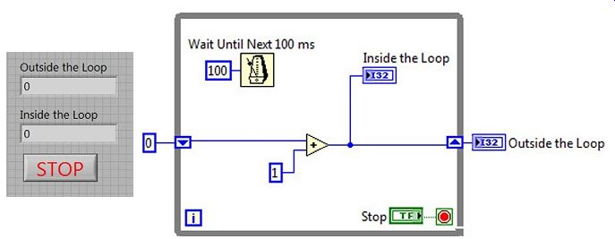
Figure 9
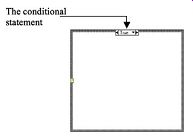
Figure 10
7. Case Structure in LabVIEW
The case structure is a programming construct that is useful in emulating a switch, similar to what appears on the front panel of a hard instrument to allow the user to select one of multiple available tasks. In terms of its appearance in LabVIEW, a case structure works much like a while loop as evident in Figure 10. However, significant differences exist between a case structure and a while loop in that a case structure performs a separate operation for each case of the conditional statement that drives this structure. The conditional statement takes a value chosen by the user at runtime from among the set of values for which the given case structure is programmed to execute. This set can be {0,1}, as is the case initially when a case structure is added to a VI, and can be expanded during the programming stage by right clicking on the conditional statement and choosing "Add case" as necessary. For each case, the VI must include an appropriate execution plan that is placed within the bounding box of the case structure. The conditional statement associated with a case structure is typically driven by a ring, which is placed on the front panel of the given VI and appears outside the bounding box of the case structure in the block diagram panel of the VI.
This ring is connected to the question mark box on the right side of the case structure in the block diagram. This is illustrated in Figure 11 in conjunction with a four-function calculator implemented in LabVIEW. It is evident in Figure 11 that the ring, acting as an operation selector, drives the condition statement, whereas variables X and Y, implemented via numerical controls on the front panel, pass their value to the case structure, which embeds the actual mathematical operation for each of the four functions (add, subtract, multiply, and divide) in a dedicated panel.
Figure 11 depicts the panel associated with the divide operation. Arrows in the condition statement of the case structure can be used during the programming stage to open each of the cases that the case structure is intended to implement. The ring outside the case structure must have as many elements as there are cases in the respective case structure. Here, it is important to make sure that the order of the selections in the ring and the order of the functions in the case structure correspond to each other. If the first option in the ring is "add," the first function of the case structure needs to implement the addition function. Exercise 6 deals with this issue at more length. Note that as is the case with other LabVIEW elements, right clicking on a given element allows the user to view a detailed description and examples associated with that element.
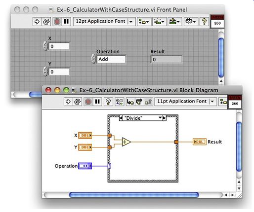
Figure 11
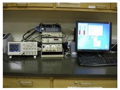
Figure 12
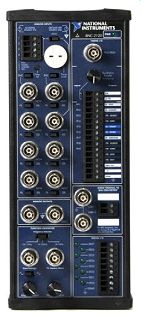
Figure 13
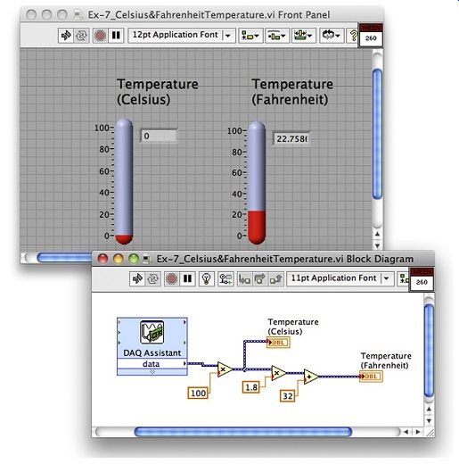
Figure 14
8. Data Acquisition Using LabVIEW
LabVIEW is primarily a data acquisition tool. The typical setup in the laboratory is shown in Figure 12. Aside from the hard instruments shown in Figure 12, which are also used to perform data acquisition and monitoring tasks, a terminal box is needed to obtain the input from sensors and to allow a way to produce output voltages from the data acquisition card.
A typical connector block is shown in Figure 13. This is National Instrument BNC-2120.
Pin numbers and the style of the terminal box will vary depending on the model being used.
The experiments described later in this SECTION use BNC-2120, but several will use different terminals. For the exercise discussed below the data acquisition card's differential mode is used, meaning that it reports the voltage difference across a channel (channel 0 in our case). The card can also operate in an absolute mode where it references the reading to the ground level. Finally, there is one last piece of equipment, which will be needed in the subsequent discussion: the function generator, which can be seen in Figure 13.
As the name suggests, this piece of equipment is used to generate a sine wave, a triangle wave, or a square wave. The amplitude of the wave can be adjusted by using the amplitude knob. The frequency of the wave can also be adjusted using the relevant buttons. The main use of this device in the present context is to produce an external input to a custom VI that is shown in Figure 14, which converts the voltage produced by the function generator into a temperature reading in Celsius and Fahrenheit units.
Functions related to communication with the DAQ card are handled by the "DAQ Assistant" function. The board ID and channel settings specify information about the DAQ card that tells the VI where to look for data. The algebraic operations that implement the conversion of data are more or less straightforward as depicted in Figure 14.
9. LabVIEW Function Generation
n this section we will create a VI that emulates a function generator, that is, the VI should produce a periodic signal with a user-selected shape, frequency, and amplitude to an output channel on the National Instruments DAQ card. In addition, the user should be able to select the resolution of the waveform (i.e., the number of data points per period). The VI's front panel should also include a waveform graph that displays at least one period of the waveform selected as it appears in Figure 15.
The VI produces a sine wave, triangle wave, or square wave as selected by the user. This requires that a case structure be wrapped around the signal generation block and a ring block to communicate between the front panel and the case structure. This is discussed further in the LabVIEW exercises at the end of the SECTION.
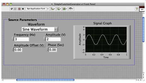
Figure 15
10. Summary
This SECTION was meant to introduce the reader to the usage of LabVIEW in computer-based data acquisition. Basic LabVIEW programming concepts, namely controls, indicators, and simple nodes used to implement algebraic operations, as well as program flow control constructs, that is, while loop and case structure, were introduced. These building blocks were used to implement increasingly more complex LabVIEW VIs. These VIs can be used as stand-alone LabVIEW programs or expanded to form sophisticated VIs in conjunction with additional LabVIEW elements. These include signal processing tools, which are discussed in the subsequent SECTION. The exercises that follow enable the reader to practice constructing a number of VIs that are of value in a laboratory setting.
11. Problems
1. In order to demonstrate your understanding, build the VI found in Figure 3. To get started, click on the LabVIEW icon found on the desktop of your computer (assuming it is previously installed). This should pop up a window with several choices. Select "Blank VI" and click "OK." From here you should see the front panel (it is gray). To open the block diagram window go to the window and then the show block diagram option (Ctrl-E or Cmd-E also do the same). On the front panel, you will need to add the required numeric controls for X and Y and numeric indicators for X + Y and X - Y. These are available in the modern subpalette of the controls palette, which is available by right clicking in the front panel. You will then use the block diagram window and implement the add and subtract nodes (available in the numeric section of the programming subpalette of the functions palette, which itself can be viewed by right clicking in the block diagram window) and connect them to the appropriate controls and indicators.
Note that you can change the labels of each entity by using the text tool from the tools palette. Changing the label of an indicator or control in the block diagram window changes its label in the front panel as well. Once you have inserted the necessary nodes and wired them together properly, you can run the VI by pressing the run button at the upper left corner of the front panel window. The digital indicators should then display the results of the addition and subtraction operations. You can also use continuous run button , which is next to the run button.
2. Create a program that will take the slope of a line passing between any two points. In other words, given two points, (X1, Y1) and (X2, Y2), find the slope of the line, Y = mX ) b, that passes through these points. This program should have four digital inputs (as numeric controls) that allow the user to select the two coordinates. It should have one digital indicator that provides the value of the slope of the line between them.
3. Using ideas similar to those in Figure 8, demonstrate your understanding of the logic operations by adding an additional indicator that will display the greater of the two numbers determined from your addition and subtraction operations in Exercise 5.1. Is the number obtained by the addition operation always the greatest?
4. Demonstrate your understanding of logic operations by building a VI that takes as input three numbers and outputs the greatest and the smallest value of the three. This will involve very similar logic operations to the one performed in the earlier VI.
5. After you have had a brief exposure to the operation of loops and other structures in LabVIEW, practice by creating the program from Figure 9. When fully operational, the program should continue to increment by a counter 1 every 0.1 seconds until the stop button is pushed. Verify that this is true and that waiting longer to press the stop button results in a larger number. What is the difference between inside and outside loop displays? Why do you think this happens? If you let the program run and forgot to turn it off when you left the lab, would your program ever be able to reach infinity? Explain your answer.
6. The specific task that you will perform is to create a calculator that will add, subtract, multiply, or divide two numbers using a case structure as depicted earlier in Figure 11.
This will require you to use two inputs, an output, and a ring on the front panel. You will need a case structure in the diagram window, which initially will have only two cases {0,1} but these can be extended by right clicking on the condition statement in the block diagram. The case structure itself can be found in the structures subpalette of the functions palette. The ring should be added to the front panel of the VI and can be found on the modern subpalette of the controls palette. The properties dialog box of the ring, which opens up by right clicking on the ring, allows you to add cases as you need (in this case, four cases). Make sure the order of the list on the ring corresponds to the case list.
7. Data acquisition is probably the most important aspect of LabVIEW. To be able to understand completely what takes place when you are taking data, it is important to know what tasks are performed by a VI that acquires data from an external source. The VI introduced earlier in Figure 14 takes a temperature measurement every time the run button is pushed. While this is useful for taking measurements where temperature is constant (e.g., room temperature), it is not useful in tracking temperature changes.
(The next exercise addresses this issue via a loop structure.) If a low-frequency squarewave is used, however, it is possible to verify that the VI functions as intended. Connect a function generator to the DAQ card. Make sure that the function generator is set to produce a square wave and that the frequency is set to be about 0.1 Hz. You may wish to view the signal on an oscilloscope to ensure that the function generator is indeed producing the desired waveform. This can be done by connecting the output of the function generator via a BNC connector to Channel A (or Channel 1) on a typical two-channel scope. Be sure to set the trigger-mode to external (EXT) and choose Channel A (or Channel 1) as the trigger source.
You may have to initially use the ground function of the scope to ensure that the beam is zeroed at the midlevel of the screen and that the vertical and horizontal scales are set up properly. The same BNC connector can be used to connect the function generator to the BNC-2120, which acts as the interface between the DAQ card and the function generator.
8. In this exercise we need to add a loop to the VI from the previous exercise so that the VI can take readings continuously until a stop button on the front panel of the VI is pushed and the VI is stopped. The loop construct is in the structure subpalette of the programming section of the functions palette. You can also find the stop button in the Boolean subpalette of the classic section of the controls palette. Verify that this works and watch how the temperature reading changes with time. Change the frequency of the function generator and observe the effects of the output. What difficulties arise when the frequency is too fast relative to the timing capacity of the loop? If we had no digital indicator, only thermometers, would this be a problem?
9. In this exercise, we will add more functions to the VI from the previous exercise. If we only want to maintain some temperature (e.g., in a thermostat), we might only care about the highest value of the temperature. Use the logic operators to determine the highest temperature of all the measurements (hint: you will need a shift register). In LabVIEW, there are many different options for data types (scalar, dynamic data, waveform, etc.).
For this part of the experiment, you will need to convert from the dynamic data to a single scalar. To do this, right click in the block diagram and select express, signal manipulation, from DDT. Then place the block, select single scalar, and then click OK.
This VI gives a little more insight into data acquisition with LabVIEW and some of the difficulties that may arise. With this VI, will you be able to tell how temperature changes as a function of time? What could we do to solve this problem (in general)? What are some of the problems with the various output styles that we have considered? What might be some more beneficial ideas?
10. Based on the function generator in Figure 15, random noise should be added to the signal by means of the "add noise" option of the signal simulation block, in the signal analysis toolbox. The output from the function generator should be added to the noise using an addition block, as it can add both signals and constants. Send this noisy signal to a new waveform graph. In order to extract the original signal from the noisy signal, a filter will be applied. The filter reduces the effect of portions of the signal that are above a specified frequency. This allows us to remove the high-frequency noise. The filter block can be found in the signal analysis toolbox. Configure the filter to remove noise from the signal. Your front panel window should look much like Figure 16.
11. Select three sets of operating conditions (i.e., amplitude and frequency) for the triangle wave pattern and measure the actual amplitude and frequency of the waveform shown on the oscilloscope. This will require you to connect the DAQ board to the scope inputs using BNC cables. Verify that your measured amplitudes and frequencies are the same as those you input to the VI. Vary the noise amplitude between 0 and twice the signal amplitude and take screen captures of the results.
12. Appendix: Software Tools for Laboratory Data Acquisition
12.1 Measurement Foundry
Measurement Foundry is produced by Data Translation and has significant capabilities for rapid application development in conjunction with DT-Open Laters for .NET class library and compliant hardware. It offers the ability to acquire, synchronize, and correlate data and to perform control loop operations. It also features automatic documentation of programs and links with Excel and Matlab.
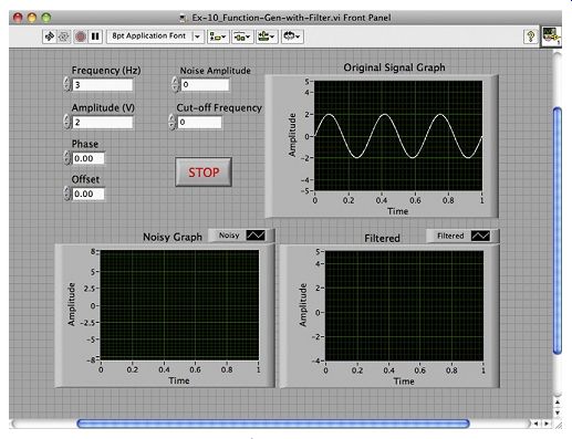
Figure 16
12.2 DasyLab
DasyLab from Measurement Computing Corporation (MCC) allows for the integration of graphical functions, real-time operations, including PID control, and real-time display via charts, meters, and graphs, and incorporates an extensive library of computational functions. It provides serial, OPC, ODBC, and network interface functions and supports data acquisition hardware from MCC, IOtech, and other vendors.
12.3 iNET-iWPLUS
This software, sold by Iomega, which is also a distributor of DAQ cards and sensors, can be used to generate analogue and digital output waveforms and run feedback/control loops, such as PID, and has capabilities similar in concept to LabVIEW, which allow for the creation of custom virtual instruments.
12.4 WinWedge
WinWedge is yet another data acquisition software that uses a Microsoft Windows Dynamic Data Exchange mechanism to provide data acquisition and instrument control in conjunction with Microsoft Excel, Access, and so on. It provides a menu-driven configuration program and is used mainly in conjunction with serial data streams.
PREV. | NEXT