AMAZON multi-meters discounts AMAZON oscilloscope discounts
1. Introduction
Analog and digital filters are used extensively in sensor signal processing. In this SECTION, both of these topics are discussed and examples using LabVIEW are presented. The main use of these signal-processing techniques is in pre- and postprocessing of sensor signals. In particular, analog filters are often used to deal with the so-called aliasing phenomenon that is common in data acquisition systems. Digital filters are generally used to postprocess acquired signals and can be used in conjunction with sophisticated digital signal-processing techniques such as Fast Fourier Transform to perform spectral analysis of acquired signals.
With this in mind, the SECTION introduces the reader to the following topics:
• Analog filters, their analysis, and synthesis using passive components (resistors and capacitors) as well as active components (operational amplifiers).
• Frequency response of a low-pass filter using Bode plots, illustrating the response of the filter with varying frequency of the input signal.
• The concept of a digital filter as counterpart to the analog filter and built using software.
• Implementation of moving average (MA) and autoregressive moving average (ARMA) model-based digital filters and their implementation in LabVIEW.
• Using LabVIEW to develop virtual instruments ( VIs) that implement digital filters and demonstrate their functioning using a graphical display of pre- and post filtered signals.
These learning objectives are illustrated through detailed descriptions, examples, and exercises.
The presentation refers to supporting hardware from National Instruments and other manufacturers (namely Analog Devices, a maker of micromechanical accelerometers and similar microelectromechanical components used as sensors in measurement and instrumentation).
The reader is expected to have access to a laboratory environment that allows for implementation of analog filters via passive and active electronic components, test instruments such as oscilloscopes and function generators, and, more importantly, access to LabVIEW for implementation of the virtual instruments discussed in the sequel. Use of a small inexpensive fan, which can be the basis for studying the impact of rotor imbalance and vibration that is filtered with a combination of analog and digital filters, is also useful. Other sources of real data can be used, however, so long as the measured signal manifests a combination of "good" and "bad" information, preferably at low and high frequencies, respectively, which can be used as the basis for the experimental component of the examples and exercises discussed in this SECTION. It is possible, however, to produce virtual sensor data using LabVIEW itself, as it is done in several of the examples, to illustrate signal processing techniques, although it is always important to use real data at some point in the process of learning to apply signal-processing techniques.
2. Analog Filters
Analog filters are used primarily for two reasons: (i) to buffer and reduce the impedance of sensors for interface with data acquisition devices and (ii) to eliminate high-frequency noise from the original signal so as to prevent aliasing in analog-to-digital conversion.
Analog filters can be constructed using passive components (namely resistors, capacitors, and, at times, inductors) or via a combination of passive and active components (transistors or, more commonly, operational amplifiers) leading to active filter designs. We consider both cases here.
2.1 Passive Filters
Passive filters are designed with a few simple electronic components (resistors and capacitors).
The basic low-pass filter, depicted in FIG. 1, can be used to remove (or attenuate) high-frequency noise in the original signal, in this case denoted by vi. The underlying assumption is that any time function can be viewed as being a combination of sinusoidals.
More exactly, any periodic function of time is approximated by an infinite series of sinusoids at frequencies that are multiples of the so-called fundamental frequency of the original signal (the so-called spectral content of the signal). Nonperiodic functions can be viewed in essentially the same way but we must allow for a continuous spectrum. For example, the original signal, vi, may be approximated by

(eqn. 1)
where Vi,1,Vi,2,Vi,3, ... are the amplitudes of the consecutively higher frequency components or harmonics of the original signal.
These higher frequency components may represent fluctuations (or, in many cases, electrical noise) that we may wish to attenuate to prevent aliasing (appearance of high-frequency components in the analog signal as low-frequency aliases of these components) and generally to present a clean signal to the DAQ system. The filter in FIG. 1 produces an output, vo, which has the same set of components (in terms of the respective frequencies) as the original signal, vi, but at reduced amplitudes:

(eqn. 2)
where Vo,1,Vo,2,Vo,3, ... . are the amplitudes of the sinusoidal components in vo. In general, Vo,1, Vo,2,Vo,3, ... . are smaller than their counterparts in the input signal, Vi,1,Vi,2,Vi,3, ... . For instance, depending on the values of R and C in the filter shown in FIG. 1, Vo,1 may be very close to Vi,1, say 98% of this value, but Vo,2 may be about 70% of Vi,2 and so forth. The reason for this is that the given low-pass filter attenuates each signal according to its frequency; the higher the frequency, the larger the attenuation (hence the smaller the amplitude of the given component in the output signal). The precise amount of attenuation can be found from the so-called frequency response graph of the filer (commonly referred to as its Bode plot) as, for instance, depicted in FIG. 2.
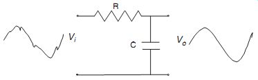
FIG. 1
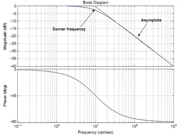
FIG. 2
The specific equation for the filter from the application of Kirchoff's current law at the output node (assuming an open circuit or no load at the output) is given by
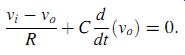
(eqn. 3)
This can be simplified into
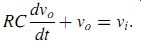
(eqn. 4)
As a first-order differential equation, it can be transformed into transfer function form, using Laplace transform, as

(eqn. 5)
where t=RC is the time constant of the filter, that is, essentially the time it takes for the filter to respond to a step input function by reaching 63% (almost two-thirds) of its steady-state output.
The inverse of t, that is, oc = 1/t, is known as the corner frequency of the filter, that is, the frequency above which the filter starts to attenuate its input. These are discussed further below in the context of the so-called Bode plot of the filter. Assuming sinusoidal functions of the form vi = Vi(ot), whose Laplace transform is given by:

(eqn. 6)
and substituting in Equation (6.6), taking partial fractions and simplification (including dropping the transient response term as detailed in the appendix), the steady-state output would be vo=Vo sin(ot)f), where
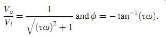
(eqn. 7)
(eqn. 8)

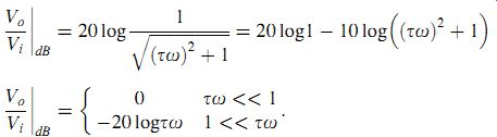
(eqn. 9)
The graph of the Vo/VijdB is precisely what was depicted earlier in FIG. 2where it is evident that higher frequencies, particularly those higher than the corner frequency of 10 r/s, are attenuated at an increasing rate, leading to the reduction of high-frequency components in the filtered signal.
2.2 Active Filters Using Op-amps
The passive filter shown previously is simple and can, in principle, be used to filter out undesirable components of a given signal. However, because it is made up of entirely passive components (resistors and capacitors), it has to draw current from the input and will, in addition, "load" the circuit connected to the output of the filter. Op-amps can eliminate this problem, as the current that is drawn from the input stage is very small (because op-amps have large internal resistances, of the order of 10 MO). Likewise, as active devices, op-amps supply current to drive their output and hence minimize the impact of the filter on any output circuit, such as the DAQ card, thereby less affecting the reading of the acquired signal. With this in mind, op-amps are often used in conjunction with resistors and capacitors to create an active filter. A sample configuration is given in FIG. 3.
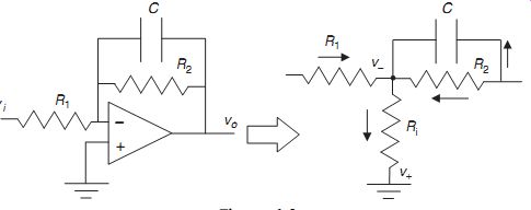
FIG. 3
To be able to utilize this circuit, we must determine the relation between the input vi and the output vo. The summation of currents at the inverting input is given by
Now, given that in a negative feedback configuration as shown earlier, v_ = v) = 0, we can simplify this to
We can rewrite this as:
This is very similar to a passive filter equation, with the exception of the gain on vi. The negative sign means that the filtered signal will lag at least 180 degrees behind the unfiltered one. (This issue can be resolved via an inverting filter of gain of +1.) We can call this gain k, so k = R2/R1. In addition, we see that the time constant is given by t = R2C. So, we have two degrees of freedom in our filter configuration. We may adjust the gain constant, k, to amplify low-frequency signals. However, this will also raise the value of the crossover frequency and therefore allow noise to have a higher amplification. In addition, we can change the corner frequency (oc = 1/t) by adjusting the relevant parameters. This will have effects on the gain as well, which must be taken into account. These can be better understood by examining the system in the frequency domain. In the frequency domain, the ratio of the output to the input voltage is given by
We can understand better how the filter works by examining the Bode plot of the system, which is indeed similar to that in FIG. 2, with the only exception being an upward shift of the graph by 201ogk. As discussed earlier, the graph is meant to illustrate how the filter passes through signals of frequency up to its corner frequency and gradually attenuates those beyond this level as depicted in FIG. 2.
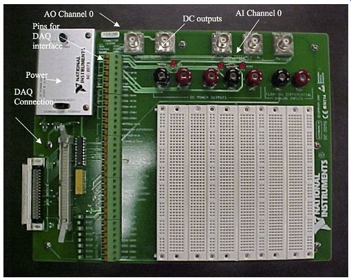
FIG. 4
2.3 Implementation on a Breadboard
In a laboratory setting, one can build and test various circuits, including low-pass filters using breadboards. FIG. 4 depicts one such breadboard made by National Instruments (NI).
Similar boards with more or less additional features are available from various manufacturers.
This particular breadboard has a connector (lower left corner) that attaches readily to an NI DAQ card. Other breadboards are also available from NI and other manufacturers.
2.4 Building the Circuit
Assuming access to a breadboard similar to FIG. 4, circuits can be built on the white section of the breadboard. The horizontal sections of holes in the wider strips of this section are connected together to allow placement of circuit components that may have different sizes, while the thinner sections provide a mechanism for access to power and ground (or common signals). In addition, as stated earlier, this particular board has the ability to interface with the data acquisition card. Inputs and outputs from the card can be taken from the pins shown in FIG. 4 and connected either to the breadboard or to external devices.
2.5 Electronic Components
variety of electronic components are used to build analog filters with resistors, capacitors being the most common types. Resistors can be either fixed or variable. As the name implies, a fixed resistor has one resistance value and cannot be changed. A variable resistor, however, can be adjusted to have different values. Resistors are coded by color as shown in FIG. 5.
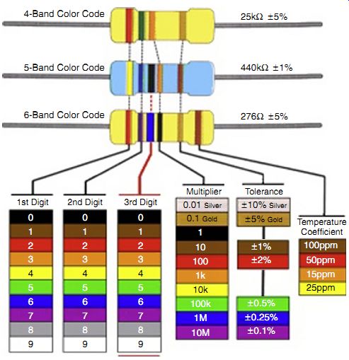
FIG. 5
Table 1 Example Resistors
Note that colors may not be evident but this same figure is generally available online at a number of sources.
Note that not all resistors have the same number of bands, so it is important to know the type of resistor at hand. If a resistor has only four bands, then it does not have the third digit. A few examples are illustrated in Table 1.
In addition to resistors, capacitors are used in building analog filters. A picture of a ceramic plate capacitor is shown in FIG. 6. Unlike resistors, capacitors have their value explicitly printed on them. Capacitance values can usually be read off in either a picofarad (pF) scale or a microfarad (mF) scale. Intermediate scales are used very seldom. In addition, it is important to note that a capacitor has some parasitic resistance as well, although this is usually very small.
Finally, op-amps are key components of analog filters. A picture of a typical op-amp, LM 741, is depicted in FIG. 7. It is important to be sure that the correct pins are used when connecting the op-amp. The data sheet for the device, generally available from the manufacturer, provides detailed specifications in this regard.
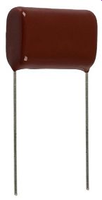
FIG. 6
2.6 Op-amps in Analog Signal Processing
As stated earlier, op-amps can be used to perform simple or more complex tasks. For instance, as shown in FIG. 8, to add two signals, vi and vr, together, an op-amp and three resistors are used. This can be useful, for instance, in adjusting for a d.c. offset in an accelerometer signal or similar cases. If we were to derive the relationships between the inputs, we would arrive at the following:
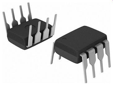
FIG. 7
Therefore, if we set vr to be the negative value of the DC offset from the accelerometer, we will be able to remove this offset successfully.
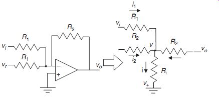
FIG. 8
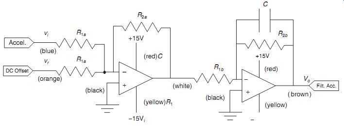
FIG. 9
More importantly, we will generally need to remove high-frequency noise in the sensor signal prior to sampling the signal with an A/D converter. For this reason, the combination of op-amps in FIG. 9 is used.
In practical implementation, color coding the wiring is helpful in preventing confusion.
Typically the coding scheme uses red, positive supply voltage; black, ground; and blue, signal.
Other colors are used to supplement these and differentiate the different signals. Exercise 6.1 refers to this in more detail in the context of performing a simple acceleration measurement experiment.
3. Digital Filters
Digital filtering uses discrete data points sampled at regular intervals. These data points are usually sampled from an analog device such as the output of a sensor (say an accelerometer used to measure vibration in a beam). Digital filters as shown schematically in FIG. 10 rely not only on the current value of the measured variable, but also on its past values (either in raw or filtered form). This leads to two kinds of filters, which are examined in the sequel.
3.1 Input Averaging Filter
In the input averaging filter, the previously unfiltered values of the given signal are used in the scheme. This filter takes the form of

( eqn. 10)
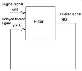
FIG. 10
Note that we can write a0 _ a and a1 _ 1- a and hence write the above as

( eqn. 11)
and thus further extend this formulation to more complex filters such as

( eqn. 12)
This general form is called a moving average filter, as it in effect averages past values of the input signal, each with its respective weight. Selection of these weights is often an issue and can be formalized, although in the present context we will deal with simpler cases in which an intuitive approach to selecting these values can be used.
3.2 Filter with Memory
In a filter with memory, previously filtered values are used to adjust the new output. This filter takes the form
yk = auk )(1 + a)yk_1;
where a is the weight on the current value of the unfiltered signal, uk. The remainder is from the previous value of the filtered signal, yk-1. Varying a will change the extent to which the input signal is filtered. In particular, a relatively large a weighs in the current value of the input signal, while a small a weighs in the past (filtered) signal, yk. Normally, a + 1.
This is evident in the following example.
3.3 Example
A set of data points is measured from a continuous signal as given in Table 6.2.
Table 2 Data for Digital-Filtering Example
A simple input averaging filter with a values of 0.25, 0.5, 0.75, and 1.0 is used to filter these values as depicted later (FIG. 11). The filters produce a continuum of response patterns indicating that no single value of a is best. However, one can argue, based on proximity to the general pattern of the input signal, that a = 0.5 may be reasonable.
In practice, one has to fine-tune a or similar parameters of a given filter to fit the application in mind. There are, as shown later, formal methods (based on digital signal processing) that allow the user to select the filter parameter to affect the frequency response of the filter (similar to the analog case). The mathematical techniques underlying these tools are beyond the scope of this guide although their application is discussed later.
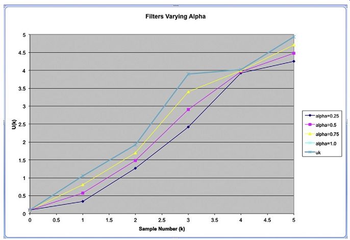
FIG. 11
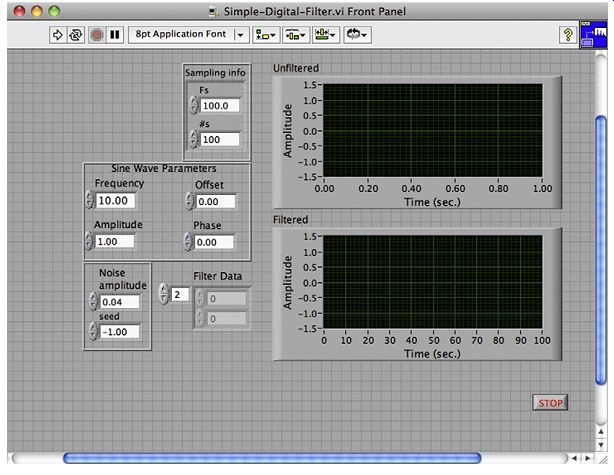
FIG. 12
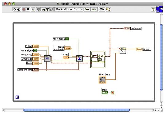
FIG. 13
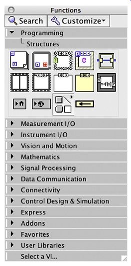
FIG. 14
3.4 LabVIEW Implementation
One can implement a digital filter in LabVIEW as shown in FIG. 12. The block diagram of this filter appears in FIG. 13. The filter parameters are set at 0.5 and 0.5 in the lower left corner of the front panel but can be changed if necessary. The block diagram depicts a sinusoidal signal generator, as well as a noise generator on the left side. The in-place operation allows the addition of individual data elements.
The in-place element structure allows a simple operation such as addition to occur on the corresponding elements of two dynamic arrays produced by the sinusoidal and noise signal generators. This node can be found in the structures subpalette of the programming section of the functions palette as depicted in FIG. 14.
[* The location of these nodes in the respective palette may change depending on the version of LabVIEW. It is, however, possible to search for a specific type of node by name and locate it irrespective of its location.]
The filter itself is implemented as a finite impulse response (FIR) filter node (found in the advanced FIR filtering section of the filters subpalette of the signal-processing section of the functions palette), which effectively implements a moving average filter type. The array of filter coefficients appears in the front panel of FIG. 12. Note that in this case the source signal is generated internally but it is possible to do the same task using an external input signal, as, for instance, generated by a function generator.
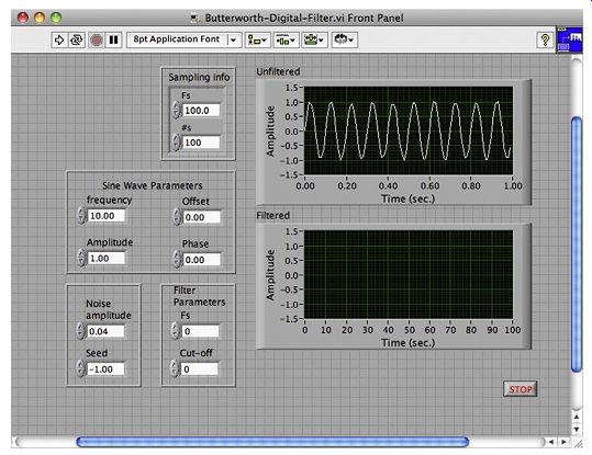
FIG. 15
3.5 Higher Order Digital Filters
While the simple filter in the previous section works reasonably well, one can build more effective filters using a combination of autoregressive terms and moving average terms, via an ARMA model, also referred to as an infinite impulse response (IIR) filter. The general equation for such a filter is given as
( eqn. 13)
FIG. 16
Note that ai and bi must be chosen properly for stable and effective performance. This is not a trivial task and requires advanced techniques that extend beyond the scope of this text. The essential idea is to place the so-called poles and zeros (the roots of the denominator and numerator of the corresponding discrete time transfer function) in reasonable locations in the complex plane. However, there are well-known design strategies that have performed well, including Butterworth, Chebyshev, and Bessel, that are programmed in LabVIEW. It is also possible to produce the filter coefficients in Matlab or a similar tool and use a similar technique as in the previous section (albeit using an IIR filter node) to implement the given filter.
Implementation using LabVIEW built-in functions is depicted in FIG. 15. Filter parameters include the sampling frequency, which in this case is the same frequency used to generate the signal in the first place. The cutoff frequency is also another required parameter, which is chosen to correspond to the frequency at which the noise components start to dominate the real signal. The block diagram is depicted in FIG. 16. The filter node (from the signal processing section of the function palette) requires filter type (set to zero for a low-pass filter) as well as the two parameters mentioned earlier. Note that the unconnected terminal of the filter node (the high-frequency cutoff) is not required for a low-pass or high-pass filter but is required for a bandpass filter.
The response of the filter depicted in the front panel diagram in FIG. 15 typifies the low-pass filtering effect of a Butterworth filter, which indeed performs better than the simple filter we designed earlier.
4. Conclusions
This SECTION considered signal-processing techniques used commonly in conjunction with computer-based data acquisition systems. As a prelude to digital signal processing via LabVIEW, we considered analog signal processing using operational amplifiers (op-amps).
This process is often essential to successful computer-based data acquisition, as the original signal may be contaminated with noise, which leads to aliasing in the digitize signal (a process akin to the appearance of ghost images on television screens). We further discussed digital filtering using moving average and autoregressive moving average models.
5. Problems
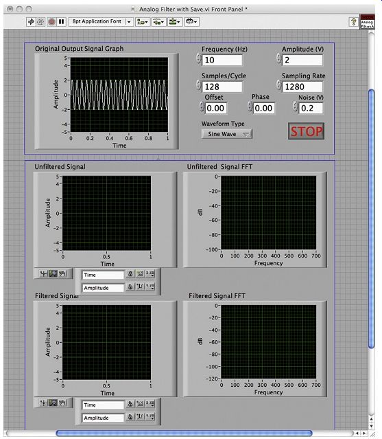
FIG. 17
1. Implement the analog filter design described in FIG. 10 using a pair of LM-741 op-amps and appropriate resistors and capacitors. You will need to choose a reasonable capacitor value for C, say 0.1pF, and then choose an appropriate resistor value for R2b to achieve a corner frequency of 10 Hz (effectively 60 rad/s). For this exercise, design the gain of your filter to be unity (1) by selecting R2a = R2b. Likewise, choose R1a = R2a because you will use the first stage only to invert the signal produced by the function generator (since it will be inverted again by the second stage filter). In building the circuit, pay close attention to the color coding marked on the figure. Do not power up the board or connect power to the circuit without first ensuring that connections are made properly.
2. Perform preliminary evaluation of the filter in the previous exercise by generating a signal using a function generator capable of producing a sinusoidal function of varying frequency (similar to that shown in the previous SECTION). You can connect the function generator output to vi input in the filter and ground vr input since it is not used in this exercise. (It is always good practice to ground unused inputs to prevent the circuit from picking up and introducing noise in the actual signal.) You will need an oscilloscope to evaluate the functioning of the filter. Vary the frequency of the signal from 1 to 100 Hz and make an estimate of the filter performance (in terms of attenuation of the signal amplitude) by recording (reading off the scope) the amplitude of the signal as a function of frequency. Compare your graph with FIG. 2. Note that the figure is drawn on a logarithmic scale. Be mindful of this fact in your comparison. Bear in mind the corner frequency of the filter, which is expected to be at 10 Hz.
3. Create the VI shown in FIG. 17. This VI can be used to evaluate the analog filter discussed in the previous exercises. The signal generated by the VI is filtered with the analog filter implemented in the previous exercises. The spectrum of both unfiltered and filtered signals is shown in the respective panels of the front panel of the VI. Set the wave type to be a sine wave, the frequency to be 10 Hz, the amplitude to be between 2 and 5 V, and the noise amplitude to be 10% of the signal amplitude.
Use an oscilloscope to verify that you are producing the correct signal. Note that the VI should be implemented such that the Analog Output Channel 0 on the National Instruments interface board is used to produce the generated signal. In addition, examine the spectrum of the signal given in the VI. Later you will want to filter the noise, not the signal. Having an idea of where the spectrum of the signal dominates enables one to filter the signal properly.
4. You can use the signal generated by the VI (via Analog Output Channel 0) of FIG. 17 with the analog filter from the previous exercises. The output of the filter should be used as Analog Input Channel 0 so you can evaluate the performance of the analog filter using the VI. Set the noise amplitude to zero in your VI. Starting with 1 Hz, adjust the frequency in steps of 2, 5, and 10, up to 1000 Hz. Determine the frequency at which the filtered wave amplitude is 1/10th the original signal amplitude.
Also, review the spectrum of the signal as it appears in the respective panel of the VI.
5. In this step, you will evaluate the performance of the filter as a function of noise amplitude. You will first set the signal frequency at 10 Hz, and set the amplitude to be 2 V. Adjust the noise amplitude from 0 to 2 V. Measure the amplitude of the filtered signal and fill in Table 3. In addition, note the impact of increasing the noise amplitude on the frequency spectrum of the filtered and unfiltered signals.
Table 3 Noise Attenuation as a Function of Amplitude
You can demonstrate further how the filter may be used in a real system. To do this you can use a small fan with a small weight attached to one of the blades with sturdy tape that prevents the added weight to fly off as the fan rotates. A semiconductor-based (MEMS) accelerometer similar to that shown in FIG. 18 may be attached to the base of the fan to record the acceleration due to an unbalanced rotor. We wish to filter out all the noise that occurs above the fan's rotational frequency. In order to do this, we must first know what the frequency is. Determine the frequency from the fan specifications, which should be available from manufacturer data sheets.
7. Create the VI for use with the accelerometer as shown in FIG. 19. The VI must be able to read the accelerometer signal and produce filtered and unfiltered displays of this signal along with the spectrum of the signal.
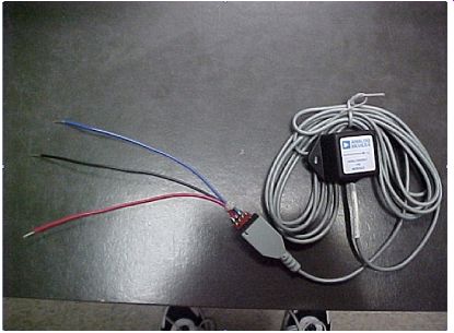
FIG. 18
8. Connect the accelerometer to the amplifier in FIG. 9. The accelerometer, in the packaging shown in FIG. 18, is manufactured by Analog Devices (and is connected readily with the filter). Examine the output of the filter on an oscilloscope to ensure that the signal from the accelerometer makes sense. Assuming that the accelerometer is attached to the base of the fan (in normally operating condition, i.e., without any added mass to create rotor unbalance) you should see the fan frequency on the oscilloscope.
The accelerometer may have an offset that can be removed in the next step.
9. Using the VI developed earlier, produce the offset necessary to eliminate the accelerometer offset.
10. Given the frequency of the fan at its high setting, calculate the corner frequency that would be needed to filter the rotational speed of the fan. You may use the same filter that you used previously or, if the corner frequency is very different, you may change your resistances to achieve a better design. In addition, you will need to increase the gain of your amplifier to amplify the accelerometer voltage and subtract off the DC offset.
11. Examine the effects of adding an imbalance to the fan. Power down the board, disconnect the balanced fan, and connect the unbalanced fan following the same procedure.
12. Modify the filter in FIG. 12 so that it allows a dial gauge to represent a, the filter parameter. This is a simple modification but allows you to better understand the filter structure.
13. Create a case diagram to allow multiple types of noise (uniform, etc.) to be added to the signal in FIG. 12. Does changing the wave type seem to have any effect on the quality of the filtered output? Does the filter reproduce each wave exactly?
14. What effect does changing the frequency have on the spectrum of filtered and unfiltered signals? What happens to the frequency spectrum of the filtered signal at high frequencies?
15. What is the effect of noise amplitude? What happens when it is small? What is the result when it gets to be the same amplitude as that of the signal, or larger? How did changing the noise amplitude affect the frequency spectrum? What information does this give you?
16. In using unbalanced fan vibration as the source of your measurements, compare the filtered responses at low and high speeds with unfiltered responses. For which fan speed is the filtered response cleaner? How does this relate to your cutoff frequency?
17. For the experiments discussed earlier the fan speeds were fairly close, so designing a filter that would be acceptable for both speeds is not very difficult. What are some of the problems with trying to use the same filter design if the two speeds are drastically different? (Hint: If the speed is low, how will the noise frequencies change?)
18. What are some potential problems of using filters in real systems? (Hint: In the earlier exercises, we knew exactly what we were looking for. What if we do not?)
19. Why does high-frequency noise get reduced in low-pass digital filters?
20. Would using more sample points in the filter be beneficial in eliminating high frequency noise? What would happen if too many points are used, that is, close to the total number of data points collected?
21. What are some potential problems of using filters in real systems? (Hint: Think if you need data in real time and a higher order filter is needed.)
6. Appendix
6.1 Simple Filter Solution

( eqn. 14)
Assuming sinusoidal functions of the form
( eqn. 15)
( eqn. 16)
( eqn. 17)
( eqn. 18)
( eqn. 19)
( eqn. 20)
( eqn. 21)
( eqn. 22)
( eqn. 23)
( eqn. 24)
( eqn. 25)

( eqn. 26)

( eqn. 27)
2. Matlab Solution to the Butterworth Filter Design
As you observed simple first-order filters may do well for eliminating random noise, but they do not do well at attenuating signals with a certain frequency. For this reason, there are many other digital-filtering approaches. Many revolve around designing an analog filter and approximating it as a digital filter. This is the case for the Butterworth filter. Luckily, this design process can be automated nicely using Matlab. Matlab uses a command called butter to generate the coefficients for a filter with a certain order and cutoff frequency. A sample command is given here.
The command just given generates a third-order Butterworth filter. The first term in the command (3 in this example) is the order of the filter. By setting this term, you can control how many past data points the filter uses. The second term in the argument is the ratio of the cutoff frequency to the Nyquist frequency. The Nyquist frequency is one-half of the sampling rate, so this ratio, r, is given by:
These frequencies are both given in Hz, which makes r a unitless quantity. It is important to note that digital filters only filter frequencies relative to the sampling frequency. If the cutoff frequency is increased and the sampling frequency is increased by the same amount, the same result is achieved. In addition, the maximum value of r is 1.0 (why do you think this is?).
However, this would correspond to an unfiltered response.
Recall that the equation for the filter is given by:
The b vector contains the b1 coefficients. The leftmost number corresponds to b0. The next number corresponds to b1 and so on. The coefficients of a are given by the next vector. Notice that our Butterworth filter has an a0 term. This isn't present in the main part of the lab. The reason for this is that the term is always set to be 1, as seen by the values of a given earlier. So, realizing that a0 is always one allows us to simplify this expression into the following:
Here are a few additional examples of Butterworth filter designs: