AMAZON multi-meters discounts AMAZON oscilloscope discounts
A microphone provides an analog output signal which is proportional to the variation in acoustic pressure acting upon a flexible diaphragm. This electrical signal is then used to transmit, record or measure the characteristics of the acoustic signal. The most common applications are related to audio broadcasting, recording and reproduction, where the frequencies of importance are in the human hearing range, 20 Hz-20 kHz. These microphones are often highly directional. This is a desirable feature when the intention is to reproduce the sound produced by a particular singer or instrument, particularly in the presence of background noise. Also, their ability to represent the measured sound level with precision is less important than their ability to reproduce the sound electrically in terms of parameters important to audio technicians, such as color, depth, warmth, etc.
Measurement microphones differ from those used for audio applications in that their primary role is to electrically reproduce the sound waveform without distortion and with a linear relationship between the voltage out and the pressure sensed by the microphone diaphragm. This precision must be maintained over a wide range of frequencies and amplitudes when measuring sound waves arriving from different angles.
Furthermore, they are expected to maintain this degree of precision over a range of temperature and barometric pressure variations.
1. Measurement Microphone Characteristics
The numerical relationship between the output voltage and the acoustic pressure sensed by the diaphragm is the sensitivity, which is expressed in units of mV/Pa. Pa is the abbreviation for Pascal, a metric unit of pressure expressed in Newton/m^2. The magnitude of the sensitivity is important in relation to the inherent electrical noise of the measurement system, since one cannot properly measure a voltage that is near the voltage noise floor of the instrument itself. Thus, for a given microphone and measurement system, the magnitude of the sensitivity will establish the minimum sound pressure, which can be accurately measured.
Any variation of the sensitivity would produce a distortion in the output signal compared to the acoustic signal. Thus, the following parameters are essential in a measurement microphone.
¦ The sensitivity should be nearly constant over the range of frequencies to be measured. Thus, a quality measurement microphone should have a "flat" frequency response.
¦ The sensitivity should be nearly constant over a wide range of sound pressure levels. This is expressed as linearity, since a constant sensitivity would pro duce a straight-line graph of output voltage versus sound pressure.
¦ The sensitivity should be nearly constant over a wide range of temperature and barometric pressure.
2. Common Microphone Types
Dynamic microphones, in which an electrical coil connected to the diaphragm is moved through an electrical field, generating a voltage proportional to the velocity of the moving element. Dynamic microphones have many characteristics that are desirable for audio applications, but they have a high sensitivity to vibration, limited dynamic range and their frequency response is generally not flat enough for measurement applications.
Piezoelectric Microphones, in which the force of the sound pressure acting on the diaphragm is transmitted to a piezoelectric element, generating a charge proportional to the applied force. These microphones are often used in very high pressure situations, such as measuring explosive blasts. Also, because of their rugged design, they find use when trying to measure small dynamic pressure fluctuations riding on top of large static pressures. In general, the noise floor of these microphones limit their use for precision sound measurement applications.
Condenser (capacitive) microphones, in which the movement of the diaphragm relative to a fixed backplane produces a variation in capacitance proportional to the deflection of the diaphragm. An electrical circuit provided in the microphone preamplifier converts the capacitance variation to a voltage variation. The characteristics of condenser microphones-high sensitivity, wide dynamic range, flat frequency response, low internal noise, low distortion and high stability-make them the design of choice for measurement microphones. Less precision versions of the condenser microphone, much less expensive to manufacture than measurement quality designs, are also commonly used in audio applications such as broadcasting and portable telephones.
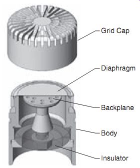
FIG. 3.1: Measurement microphone, cut-away view.
3. Traditional Condenser Microphone Design
FIG. 3.1 presents a sectional view of a typical condenser microphone showing details of the mechanical elements.
The diaphragm, a thin metal sheet stretched and clamped over the body of the microphone, deflects with the variation of air pressure about the atmospheric value. A stainless steel backplane makes up the other plate of a capacitor, whose capacitance varies as the diaphragm is displaced in response to sound pressure variations. The precision required to produce a microphone of measurement quality is extreme; the diaphragm thickness will be in the range 1-2 µ-inch and the space between the diaphragm and the backplane will be on the order of 0.001 inch.
In the conventional condenser microphone, a highly stable DC polarization voltage, also referred to as the bias voltage, is applied between the diaphragm and the backplane which generates charges of opposite polarity on them. Variations in the spacing between the diaphragm and the backplane resulting from the action of the acoustic field result in proportional variations of the difference in voltage between them. In practice the microphone is threaded onto a cylindrical preamplifier of the same diameter containing an electrical circuit that has an ultra-high input impedance. The polarization voltage is typically 100-200 volts, although lower levels in the 25-35 volt range are sometimes used to reduce the sensitivity of the microphone or to minimize the potential for electrical breakdown in the air gap when working in high humidity environments.
The dynamics of the condenser microphone can be modeled as a spring-mass-damper system, where the diaphragm is the mass, the tension in the diaphragm the spring and the damping is provided by air friction in the space between the diaphragm and back plane. The frequency response is therefore flat up to a relatively high frequency where the effects of the resonance of this mass-spring-damper system begin to be seen. The lower frequency is controlled by the size of the vent opening, which is necessary to equalize the interior of the microphone to variations in atmospheric pressure. The majority of applications of condenser microphones are at frequencies well above the low frequency -3 dB point, which is typically a few hertz.
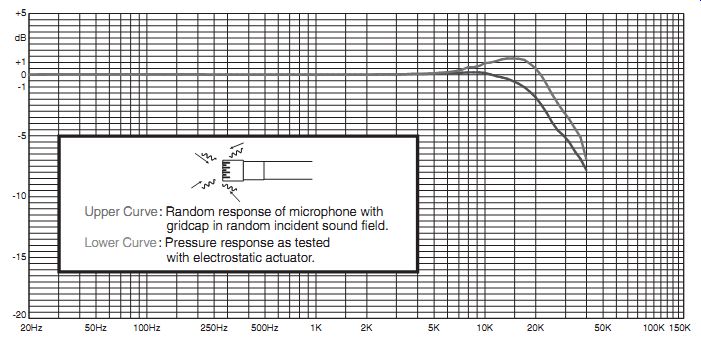
FIG. 5.1: Frequency response of ½" microphone using an electrostatic
actuator (lower curve).
Effect of Angle of Incidence of Sound Wave
The electrostatic actuator simulates the action of a pure pressure variation uniformly distributed across the surface of the diaphragm. This is called the pressure response of the microphone. In practice, one situation in which the diaphragm might be excited by a uniform pressure is when the microphone is sensing the pressure within a cavity whose dimensions are much smaller than a wavelength of the exciting frequency.
In this case, there is no wave motion and the pressure varies uniformly throughout the cavity as a function of time. However, in most sound measurement situations, the pressure driving the diaphragm is the result of one or more sound waves impinging on its surface from various directions.
An acoustic wave generates both pressure variations and local particle motions in the fluid medium. In certain circumstances, the particle velocity is in the same direction as the propagation of the wave and also in-phase with the pressure variation. One of these situations is when a wave is propagating within a tube whose diameter is much less than the wavelength of the wave. Another is when the wave is generated by a single source in a free and empty space (no reflections) and the measurement is being made at a distance far from the source. We refer to these as plane waves and we can use them to illustrate the effect of angle of incidence of the response of the micro phones.
Pressure Microphones
Consider the situation in the acoustic free field where a sound wave from a single source is approaching the microphone in a direction parallel to the surface of the diaphragm.
The angle of incidence is defined as relative to the direction normal to the surface of the diaphragm, so this situation is referred to as 90º incidence. The wave moves smoothly across the diaphragm without reflection, so the diaphragm is driven only by the pres sure associated with the traveling wave. For this reason, the microphone design we have been describing is referred to as a pressure microphone. At low frequencies, where the wavelength of the sound is much larger than the diameter of the microphone, the pressure across the surface will be essentially uniform. However, at higher frequencies, as the wavelength of the sound decreases, the pressure across the diaphragm becomes non uniform, eventually leading to with areas of positive and negative pressure at very high frequencies, as shown in FIG. 5.2.
The overall effect of this is a diminishing force on the diaphragm. As a result, the frequency response of the microphone will drop-off at higher frequencies, as shown by the 90° incidence curve on the right in FIG. 5.3, limiting the upper frequency limit of the flat response portion of the curve, and thus the useful measurement range of the microphone. Since this effect is based on the diameter of the microphone as a function of the wavelength of the sound, the upper limit of the useful frequency range of this type of microphone is higher for smaller diameters.
If we rotate the microphone so that the wave strikes the surface of the diaphragm as shown by the 0° incidence diagram on the left of FIG. 5.3, this effect will not occur because the pressure will be uniform across the face of the diaphragm at all frequencies. However, because the diaphragm is solid, it is necessary that the particle velocity at the diaphragm surface be zero, which is accomplished by the presence of a reflected wave propagating back in the direction towards the source (this phenomenon only occurs at higher frequencies). The result is an increase in the pressure seen by the diaphragm. The curve labeled 0° in FIG. 5.3 illustrates how this reflection affects the shape of the upper end of the flat region of the frequency response of the microphone as a function of frequency. The effect of this reflection for other angles of incidence is less pronounced, as shown in FIG. 5.3.
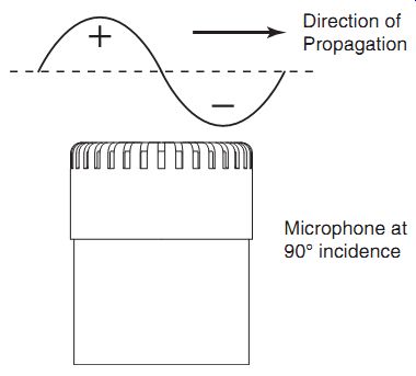
FIG. 5.2: Wave traversing microphone diaphragm, 90º incidence.
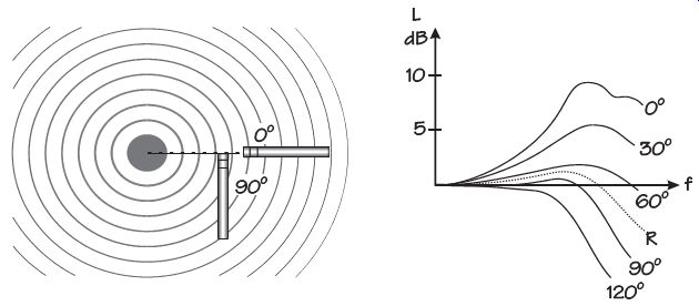
FIG. 5.3: Free field corrections.
For most microphone designs, this 0° free field correction can be calculated mathematically by modeling the microphone as a cylinder whose axis is aligned with the direction of propagation of the incident sound wave. To determine the frequency response of a particular microphone for waves approaching from any angle, the free field correction for that angle is added to the frequency response obtained using an electrostatic actuator. We refer to the frequency response of the microphone for 90° incidence as the pressure response, and for 0º incidence as the free field response.
Free Field Microphones
Note that the effect of the reflection from the diaphragm at 0° degree incidence is to increase the frequency at which the curve drops off, although the departure from the flat response makes this frequency region unusable for measurement purposes. By modifying the microphone design to increase the damping, it is possible to reduce the amplitude of the peak associated with the refection, thereby increasing the upper limiting frequency of the flat region of the curve. This creates a new type of microphone, the free field microphone, which measures best when oriented such that the wave is approaching with 0° incidence. The microphone is designed to compensate for its presence in the sound field.
In FIG. 5.4, we see the typical pressure (electrostatic actuator curve) and free field response of a free field microphone.
FIG. 5.5 shows the directional characteristics of a free field microphone in a polar format, along with the same data for a sound level meter using this microphone.
The effect of the body of the instrument can be clearly seen for sound waves approaching from angles greater than 90°.
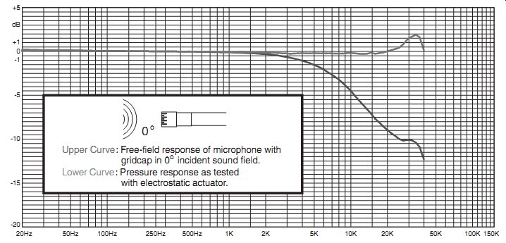
FIG. 5.4: Free field microphone frequency response.
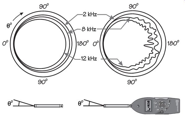
FIG. 5.5: Directionality of a ½" free field microphone, alone
and mounted on a sound level meter.
From this data, we can see that when using a free field microphone to measure the sound generated by a single source in a free field, the best measurement is obtained by aiming it towards the source, at 0º incidence. When using a pressure microphone, however, the best measurement is obtained by orienting the microphone axis perpendicular to the direction of wave propagation, at 90° incidence.
The main situations where a measurement is made of a single sound source in a free field are as follows:
1. In an open space outdoors, far from other noise sources.
2. Inside an anechoic chamber, a specially designed test room whose surfaces are covered with long, acoustically absorbent wedges designed to trap and absorb incident acoustic waves.
Random Incidence Microphones
In most acoustic measurement situations the microphone is exposed to sound waves approaching it from many directions. This could be due to the presence of multiple sound sources, moving sound sources, or the result of waves reflected from nearby hard surfaces as is common with indoor measurements. When using a microphone under such conditions, where impinging sound waves could be arriving from a variety of directions that might be varying with time, we define a random incidence correction in a similar manner to the free field correction. To determine this, measurements are performed in an anechoic environment using a single sound source to determine the frequency response of the microphone using angles of incidence over a 360º range, in steps of approximately 5°. Assuming that the waves arrive with equal probability over this range, a mathematical calculation can produce the frequency response which would have been obtained had it been possible to actually simulate such a test.
The procedure for determining the random incidence response of a microphone is described in the international standard IEC 1183 (1994) Electroacoustics-Random incidence and diffuse-field calibration of sound level meters. The result is a frequency response curve lying between the pressure and free field response curves, as indicated by the curve labeled R in FIG. 5.3. For a pressure microphone, the random incidence response will be fairly close to the pressure response so these are often used in random incident measurement situations. The upper curve in FIG. 5.1 represents the random incidence frequency response of a ½ " pressure microphone.
The design of a pressure microphone can be modified to provide a frequency response that is optimized for random incidence measurements. Free field microphones, however, do not generally have an acceptable random incidence response.
Thus, a particular measurement microphone will be designed for use under one of the following acoustic field conditions:
¦ pressure
¦ free field
¦ random incidence
In many cases pressure microphones having diameters of ½” or less are designated as both pressure and random incidence microphones since their frequency response characteristics are satisfactory for use in both types of acoustic fields.
6. Limitations on Measurement Range Lower Level Limits
In addition to the limitations on useful frequency range described above, there are also limitations on the sound pressure level, in dB, over which an accurate measurement can be obtained. The lower measurement limit of the microphone is established by its cartridge thermal noise. This is the dB level that would be read by a measurement instrument connected to the microphone output when there is no acoustic pressure applied to the microphone. There are two sources of thermal noise, air damping and preamplifier circuitry. The air damping causes a white noise that is a property of the microphone. The preamplifier has low frequency noise which is inversely proportional to frequency as well as white noise. In general, larger microphones have lower thermal noise, so they are often used for measurements of low noise levels.
Upper Level Limits
Mathematical modeling of the dynamics of the condenser microphone shows that the dynamic response in terms of output signal to capacitance variation is slightly nonlinear.
This produces distortion in the output signal that increases at higher amplitudes. The upper measurement limit is established as the amplitude, in dB, for which the total harmonic distortion of the output signal exceeds 3%, a level that can be calculated analytically for a particular microphone design. The actual limit is not only dependent upon it's physical limitations, but it is effected by both the sensitivity of the microphone (mV/Pa) as well as the output voltage of the mated preamplifier. Lower sensitivity microphones can typically measure higher decibel levels.
Effect of Diaphragm Tension
The dynamics of a microphone are strongly influenced by the tension applied to the diaphragm during manufacture. A looser diaphragm will deflect further for a given pressure excitation, producing a greater sensitivity. However, it will also reduce the upper frequency limit and the upper amplitude limit. Most manufacturers of condenser microphones produce two versions of ½” diameter microphones, the one with the looser diaphragm being referred to as a high sensitivity microphone.
7. Effect of Environmental Conditions
The sensitivity of a condenser microphone can be influenced to some degree by variations in temperature, humidity and barometric pressure. Microphone standards require that the manufacturer specify these variations. More significantly, as will be explained in more detail later, sound level meter standards establish maximum permitted variations in performance over specified ranges of temperature, humidity and barometric pressure. Since the microphone is the component having the major influence on these variations, this in effect establishes required performance specifications in terms of temperature, humidity and barometric pressure on the microphone that is to be used with the sound level meter.
Typical Performance Specifications
The most common types of microphones commercially available have diameters of 1”, ½” and ¼”. These are generally available in pressure, free field or random incidence designs. And, as mentioned above, ½” microphones are often available in standard and high sensitivity versions. Typical performance specifications are as follows:
* Based on frequency response variation within ±2%.
8. Microphone Standards
Microphones used for test and measurement purposes are governed by the international standard IEC 1094-4, measurement microphones-specifications for working standard microphones (IEC stands for International Electrotechnical Commission). This standard establishes the parameters that must be measured and provided by the manufacturer. In addition to those presented above, this standard requires the reporting of the following specifications:
¦ Effective front volume
¦ Linearity range
¦ Static pressure coefficient
¦ Temperature coefficient
¦ Relative humidity coefficient
¦ Pressure equalizing time constant
¦ Long-term stability coefficient
¦ Short-term stability coefficient Sound Level Meter Standards
One of the main uses of measurement microphones is as the sensing element on precision sound level meters. The two standard organizations whose standards dominate the design and utilization of sound level meters are:
¦ International Electrotechnical Commission (IEC)
¦ American National Standards Institute (ANSI) These standards are the following:
¦ IEC 61672-1 (2002-05) Sound Level Meters-Part 1: Specifications
¦ IEC 61672-2 (2002-05) Sound Level Meters-Part 2: Pattern Evaluation Tests
¦ ANSI S1.4-1983 (R2001) with Amd. S1.4A 1995 Specifications for Sound Level Meters
¦ ANSI S1.43-1997 (R2002) Specifications for Integrating-Averaging Sound Level Meters
While many items in these standards deal with meter characteristics, such as detection and averaging of signals, certain others such as acoustic frequency response and directionality specifications involve the microphone directly, since it is the element of the meter which has the predominant influence on them. The ANSI standards are largely followed in North America while Europe and much of the rest of the world follow the IEC standards. In many respects, particularly those relating to signal processing, the specifications are very similar. However, there is a great divergence concerning acoustic frequency response specifications, which are mainly determined by the microphone alone.
The specifications of IEC 61672-1 require the sound level meter to have a very flat frequency response over a specified range of frequencies for sound waves impinging on the microphone diaphragm at 0º incidence, but they are not too demanding on the variation from that response for waves approaching the microphone from other directions. Conversely, ANSI S1.4-1983 (R2001) and ANSI S1.43-1997 (R2002) require the frequency response averaged over all angles of incidence to be quite flat while they are less demanding then IEC 61672-1 on the response associated with 0º incidence.
As a result of these differences, for a particular sound level meter to meet the IEC standards, it should use a free field microphone but to meet the ANSI specifications it should use a random incidence microphone. It also means that a sound level meter equipped to meet the IEC standard will measure most accurately when measuring a single source with the sound level meter "pointed" towards the source and less accurately when measuring in a space having multiple sources or reflections of waves from room surfaces.
For obvious reasons, the sound level meter equipped to meet the ANSI standard will measure more accurately in multiple source or diffuse field situations than one equipped to meet IEC standards.
When there is only one source, the ANSI meter will measure less accurately than the IEC meter, but an issue is how to orient the random incidence microphone to measure as accurately as possible. Examination of the frequency response as a function of incident angle indicates that the meter should be oriented such that the sound waves from the source strike the microphone diaphragm at a angle in the range 70°-80° in order to provide the best measurement.
In practice, the selection of a microphone is as simple as deciding whether the best measurement is desired, or the ability to state that the measurement was made using a sound level meter that meets the specifications of a particular standard. In some cases an application standard may require that the measurement device meet an IEC or ANSI standard. Otherwise, select the microphone type based on its functional specifications and orient the microphone appropriately.
These standards also define several classes of sound level meters, two of which are Class or Type 1 (precision) and Class or Type 2 (general purpose) based on accuracy (at this moment ANSI uses the designation Type but IEC switched from Type to Class in the most recent update of the standard). This has led to situations where users refer to microphones as Type 1 or Type 2 when in fact this designation refers to sound level meters, not microphones. This can essentially be taken as a way of defining the ac curacy of the microphone in question in terms of whether it could be used on a sound level meter that is to meet the accuracy requirements of Type 1 or 2.
9. Specialized Microphone Types Sound Intensity Microphones
A single microphone can measure only the sound pressure at its surface. A technique called sound intensity measurement permits the measurement of the energy flow in a defined direction. This is accomplished by using a pair of closely spaced measurement quality microphones and outputting their signals to a dual channel analyzer capable of measuring the cross-spectral characteristics of the two signals. FIG. 9.1 shows a typical sound intensity probe used for these measurements.
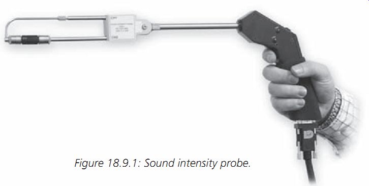
FIG. 9.1: Sound intensity probe.
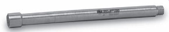
FIG. 9.2: Array microphone.
A detailed description of the technique is beyond the scope of this SECTION, but it is appropriate to comment on the microphones used for this measurement. The measurement of the phase between the signals is one of the most important parameters in the determination of sound intensity. To obtain good results, it is essential that there be a very low phase difference between them. For this reason, sound intensity microphones are generally sold in phase-matched pairs. Another feature is that their protective grid caps incorporate a small threaded stud in the center to permit them to be connected to both ends of a spacer, which holds them securely apart at a known distance.
Array Microphones
There is a growing interest in the use of measurement techniques such as acoustic holography in which simultaneous time recordings are made of the signals from a large number (16+) of microphones arranged in a fixed array. Obviously cost becomes an important issue when using such a large number of microphones, yet precision in frequency response and phase-match must be maintained to provide sufficient accuracy.
Small size is also important to minimize the interference of the microphones on the sound field being measured. Usually the microphone capsule and the preamplifier are integrated into a single unit that can easily be fixed into a support frame defining the physical arrangement of the microphones in space. The microphones are of a pre-polarized type to eliminate the need for a bias voltage and the internal electronics of the preamplifier are ICP®-powered, a technology commonly used for accelerometers with integrated circuits where an external current source of 2-4 mA provides the power.
Modern versions offer TEDS (Transducer Electronic Data Sheet) technology, in which technical specifications including sensitivity, manufacturer, model and serial numbers and calibration information are stored internally in digital format. This permits measuring instruments having the capability to read TEDS data to utilize such information automatically in creating a measurement setup, making it unnecessary to manually enter the sensitivity for each microphone, for example.
Probe Microphones A probe microphone is essentially a small diameter condenser microphone having a rigid cap instead of a diaphragm with a threaded opening into the space between the diaphragm and the end cap permitting the attachment of a small diameter hollow probe tube.
The tubes have a diameter of approximately 1.25 mm and can have a variety of lengths, typically in the range 25-200 mm. The long, narrow tube is used for measurements in small enclosed spaces, in hard-to-access areas and in the acoustic near field where the small size and high acoustic impedance of the probe have a minimum effect on the sound field. Since the tubes are usually made of stainless steel, measurements can be made in areas where the temperature is as high as 800°C (as long as the temperature inside the microphone and preamplifier housing is maintained below specified maximum limits). Although the presence of the tube causes the frequency response to begin rolling off above 300 Hz, the roll-off follows a smooth curve up to 20 kHz. This permits the use of correction curves, either supplied by the manufacturer or determined by a calibration procedure, to calculate the sound pressure level at the probe tip based on that measured by the microphone element within the body of the probe microphone assembly.
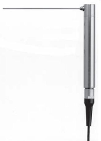
FIG. 9.3: Probe microphone.
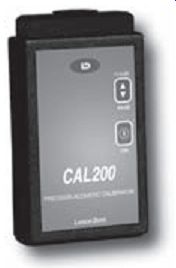
FIG. 10.1: Sound level calibrator.
10. Calibration Sound Level Calibrators
A very useful device when working with microphones is the battery powered sound level calibrator, such as shown in FIG. 10.1.
It has an internal speaker, which is electrically driven at a fixed frequency, typically 250 Hz or 1 kHz, at a feedback-controlled voltage level such that a microphone inserted into the opening in the calibrator will be exposed to a constant sound pressure level, typically 94 or 114 dB.
Pistonphone Calibrator
A pistonphone is a mechanical device in which a vibrating piston generates an acoustic pressure field within a cavity at a particular frequency, typically 250 Hz, having a fixed sound pressure level, typically 124 dB. When a microphone is partially inserted into an opening in this cavity, its diaphragm will be exposed to this same sound pres sure level. The acoustic output level generated by a pistonphone is a function of the barometric pressure, so the value is specified for measurements made at sea level.
When using a pistonphone, it therefore necessary to measure the barometric pressure at the measurement location and correct the specified output level of the pistonphone to compensate for the effect of atmospheric pressure variations from the sea level value.
Insert Voltage Calibration
Most manufacturers utilize a calibration procedure referred to as insert voltage calibration to determine the open circuit sensitivity of the microphones they produce.
In this procedure, an electrical generator is connected between ground and the diaphragm material, a digital voltmeter is connected between the backplane and ground, and a sound level calibrator is placed over the microphone. Two measurements are made. In the first, the sound level calibrator is switched on to apply an acoustic signal of known amplitude and frequency to the microphone and the output voltage is measured. Then, with the calibrator still in place over the microphone, but switched off, an electrical signal is applied to the microphone and the output adjusted until the volt meter reads the same voltage as had been read when the calibrator had been exciting the microphone acoustically. These measurements permit the calculation of the open circuit sensitivity of the microphone.
Field Calibration
The open circuit sensitivity is the sensitivity that would on be obtained if the micro phone were used in conjunction with a preamplifier having infinite input impedance.
In practice, however, the input impedances of microphone preamplifiers are not infinite and vary between different types and models. As a result, the sensitivity of the combined microphone and preamplifier may differ from the open circuit sensitivity by as much as 0.25 dB. In order to obtain an accurate measurement using a particular microphone and preamplifier, it has become standard practice before each measurement session to use a sound level calibrator or pistonphone and adjust the measurement system, or sound level meter, to read the dB output level specified for the calibrator.
With modern sound level meters and measurement systems, a corresponding value of sensitivity can be determined and tracked over time to identify changes in the sensitivity of a microphone which can be indicative of problems.
Reciprocity Calibration
A condenser microphone displays reciprocal dynamic behavior, meaning that a time varying electrical signal applied between the diaphragm and the backplane will cause the diaphragm to vibrate and generate an acoustic output having a similar waveform, just as a time-varying acoustic pressure generates an electrical output having the same waveform.
Ono Sokki 1-16-1 Hakusan, Midori-ku Yokohama 226-8507 Japan www.onosokki.co.jp
PCB Piezotronics, Inc. 3425 Walden Ave. Depew, NY 14043 www.pcb.com
References and Resources
1. C. M. Harris (ed), Handbook of Acoustical Measurements and Noise Control, 3rd ed., McGraw-Hill, New York, NY 10020, 1988.
2. Leo L. Beranek (ed.), Noise and Vibration Control, McGraw-Hill, New York, NY 10020, 1971.
3. Allan D. Pierce, Acoustics, An Introduction to Its Physical Principles and Applications McGraw-Hill, New York, NY 10020, 1981.
4. F. J. Fahy, Sound Intensity, Elsevier Applied Science, London and New York, 1989.
NEXT: Strain Gages
PREV: