THIS ARTICLE FINDS ITS ORIGINS in something I wrote in one of the early issues of TAA, all of 18 years ago (1972).
Since then, I have come back to the subject of the RIAA curve on a number of occasions, notably in 1973 in an Audio Fundamentals feature in TAA and yet again in 1977, in the British magazine, Hi-Fi News & Record Review.
So why, you may ask, am I taking it out of the drawer once more and dusting it off? Despite my view that analog records are truly dead, those that will be around for many decades will still need replaying, my own large collection included. Naturally, we aim for maxi mum fidelity, but among possible defects there is no excuse for inaccurate RIAA equalization. I must add a disclaimer. To be honest, I feel there is little point in aiming for ultra high accuracy, bearing in mind the levels of amplitude error that exist elsewhere in the chain.
-----------
ABOUT THE AUTHOR: Our Contributing Editor has been designing audio hardware for over 35 years. He has been contributing to TAA since its inception 20 years ago. An engineering executive with the telephone utility "British Telecom"; in 1985, after over 40 years unbroken service (apart from a short spell in the Army), he decided to take his pension, complete with a medal and citation from the Queen. Now, with his increased leisure time, he indulges his passion for music, good food and wine. However, he also teaches electronics part-time at the University of Keele in Staffordshire, England, attempting to convey to a younger generation some of his enthusiasm for sticky technical problems, which burns as brightly as ever.
----------------
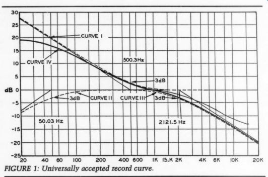
FIGURE 1: Universally accepted record curve.
The cartridge itself is the prime of fender. The most expensive high end product in the world will probably have a “spread” or amplitude deviation more than ten times greater than that likely in an equalized input stage, even though designed with a tolerance as tight as one decimal place. But before you tweakers send off those angry letters of disagreement, let me also add that provided it is not in conflict with cost-a very important consideration for a manufacturer--there is no reason why the home tweaker shouldn't aim for as much accuracy as possible. I see it as my responsibility to provide you with the technical know-how.
Origin
So, how did this all begin? Briefly, it was a reader's query on how to check the accuracy of his replay input (TAA 3/71, p. 22). I quickly designed an in verse RIAA network that would deliver an accurate low-level, fully pre-emphasized signal to the input of his replay amp. This modest contribution turned out to enjoy popularity far beyond my expectations. Yet, at the time, I thought nothing of it. It didn't involve much in the way of mathematics.
Most of the necessary equations had already been done in 1957 by W. H. Levy of EMI, and since I am not one for re-inventing the wheel, I used this in formation. Since then, Peter Baxandall presented further design information with characteristic clarity in the Radio, TV and Audio Technical Handbook published by Newnes-Butterworth in the UK in 1977 (out of print, I'm sorry to say).
In TAA 1/80, pp. 22-24, fellow contributors Stanley Lipshitz and Walt Jung also examined my original design and, apart from minor details, gave it their qualified approval.
[This became the Old Colony inverse RIAA kit, KL-3 -Ed.]
Stanley's paper to the AES in 1978, available as Preprint 1424, is mandatory reading for anyone keen on an in depth mathematical study of the whole subject.
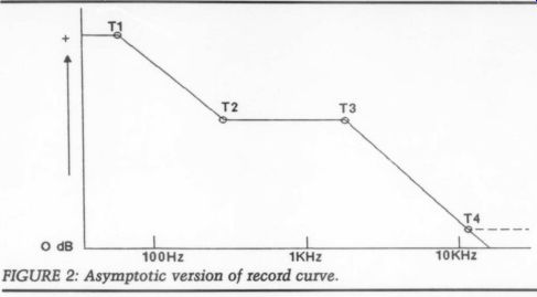
FIGURE 2: Asymptotic version of record curve.
A few weeks ago, one of my students asked a question that triggered further thinking, since it was obvious he just didn't understand the subject at all.
Like most of his generation, he believed every problem would be solved by dig ital means, but I knew better. So, I decided to do a refresher on it.
Why Equalize?
I had to deal first with a basic question from him. I offer my apologies to those readers who are already well aware why equalization is necessary at all. My student wanted to know why the analog waveform on the disc cannot be re corded to an inherently “flat response.” Well, to record the entire frequency spectrum to a constant amplitude-so there is no infringement with adjacent grooves at any frequency at peak amplitudes-is quite possible. It's when you want to play it back, you run into problems.
All cartridges available today with any claim of high quality are velocity sensitive, with the exception of crystal types. These are amplitude sensitive, and at one time, they were attractive to manufacturers of low end products simply because they had a high output and didn't require much if any equalization. With a continuous constant amplitude cut, the velocity of the groove rises in direct proportion to frequency. Replay this with a modern magnetic cartridge, and you get a rising frequency response at 6dB/octave or 20dB/decade. When you come to equalize this, you run into a number of practical design difficulties.
Over the full spectrum of say, 20Hz to 20kHz, we'd have a slope of + 60dB - - a lot of equalizing to handle. If that isn't enough, there are other problems.
Fortunately, the real world of sound comes to our rescue. It was established over half a century ago, that you didn't have to record with what amounted to constant amplitude over the entire bandwidth; part-usually in the mid to upper spectrum-could be wholly or partially constant velocity. Before long, each record company had developed its own favorite record curve, and it followed that the well-tailored hi-fi preamp of 25-30 years ago had to have selectable switching for these varying curves. Inevitably, some order was needed, to end this anarchic situation, and the ultimate outcome was a universally agreed upon record/replay curve.
Break Frequencies This curve is now embodied in internationally accepted standards. In Europe, there is the CCIR Fine Groove replay standard; in the UK, the British Standards Institution 1928:1955, amended 1965, and that in the USA, the RIAA.
Figure 1 shows the full curve and Fig. 2 an asymptotic version (a fancy way of saying, | have taken out the bends where the changes take place from constant velocity to constant amplitude and vice versa).
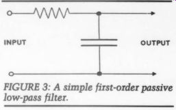
FIGURE 3: A simple first-order passive low-pass filter.
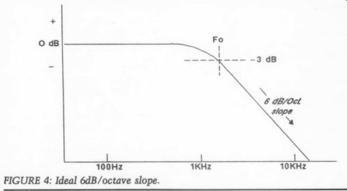
FIGURE 4: Ideal 6dB/octave slope.
You can see right away that the equalization spread required is a little under 39dB-well within practical design constraints. The equalization points are designated by the time constant of a first order filter required to produce the needed fall in response. There are three points: at 3,180uS, 318uS and 75uS.
These can be computed into “break” frequencies, where the response is - 3dB down, using the simple formula in Fig. 3 and as illustrated in Fig. 1. This yields frequencies of 50.05, 500.5 and 2,122.06Hz. Up to T1, the response is constant velocity and up to T2 it is constant amplitude with a plateau between T2 and T3 reverting to constant velocity again. Finally, from T3 onwards, it becomes constant amplitude again. I'll mention T4 later.
So, how do we go about equalizing this signal from the cartridge? It is entirely possible to do it with an individual first-order passive based on that in Fig.
3, which produces the ideal of a 6dB/oc tave slope (Fig. 4), if the input source Z is near zero ohms and the output load as near infinity as possible. I need hardly stress, the design requirements to attain these conditions leads us to some very uneconomic problems. Notwithstanding, those who regard any form of negative feedback as a bad thing have attempted it, but this is not the way it is normally done.
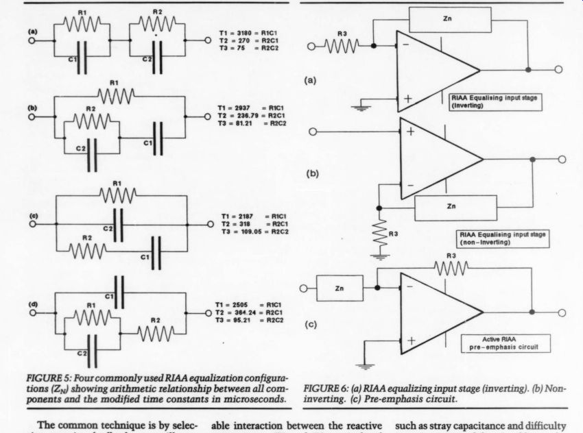
FIGURE 5; FIGURE 6: (a) RIAA equalizing input stage (inverting). (b) Non-inverting. (c) Pre-emphasis circuit.
The common technique is by selective negative feedback, as we'll see.
There is a small argument in favor of a mix, such as equalizing by negative feedback for T2 and below; then above, equalizing T3 by passive means.
Frankly, I prefer the more common, practical and economical technique of using a complex network in a feedback loop, so long as it is done properly.
Component Interaction This leads me naturally on to Fig. 5, where I have illustrated four of the complex networks that can be used in the feedback path. As a matter of interest, it was Fig. 5(b) I used in my original answer to our reader's question, back in 1971. Figures 5(a) and (b) have proven popular with designers. Though I have yet to see (c) and (d) actually used, I have included them for completeness.
The first thing we notice is that sometimes, the time constant (TC) is not what the standard apparently demands. The reason is, in a complex network of this kind, there is unavoidable interaction between the reactive components. T1 and T3 are isolated from one another in (a) but there is interaction for T2, so mathematically, you must correct this. Using the arithmetic relationship I have given, finding actual values is fairly simple. Since R2 in every case principally determines the mid band gain, you can select it first-but not before deciding which particular circuit you prefer.
Figure 6(a) has significant practical disadvantages. Since the ratio of R3 and R2 essentially determines the midband gain, in a practical version of (a), R3 must also be the load resistor for the cartridge, since it is a virtual ground at the invert input, and we know that in most cases, we require something like 47-50k. I am mainly referring to high source Z cartridges or low Z moving coils used with a transformer. To get any appreciable overall gain, R2 and the other component values are likely to be awkward, with very high R and low C.
Try it yourself and you will see what I mean. This can lead to other problems, such as stray capacitance and difficulty in maintaining stability. In addition, the cartridge itself is directly within the feedback path, which may affect circuit behavior. This factor is often over looked. It is not without good reason that (b) is usually the preferred choice and Fig. 7 shows two typical (but not definitive) examples. I have included Fig. 6(c) since it provides the inverse function of RIAA pre-emphasis. You might find it useful.
Network Design
And last, but by no means least, the net work design itself. Having, I hope, persuaded you to use Fig. 5(b), I have writ ten a short program as a design aid (Fig. 8). Right away you will see that it looks a trifle alien. Here in the UK and in Europe generally, IBM and its cloned hardware does not enjoy the market supremacy as a home PC that it does in the US. In Europe, particularly in Germany, we prefer the Atari ST. There are dozens of them at my University and I created this entire article with it, including graphics.
Our music department has just issued its first compact disc of electroacoustic music composed by members of the faculty and all created on the Atari ST.
Finally, there are a range of emulators now available, to allow access to soft ware for the Macintosh, IBM compatibles and even the obsolete CP/M. I hasten to add of course, I have no stock in Atari.
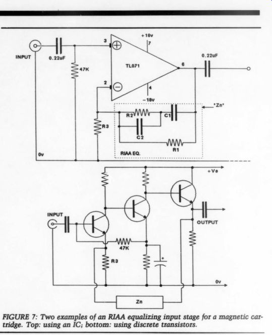
Fig. 7
This program is written in a variant of BASIC, called Fast Basic (and it is, too). There are no line numbers; they are not needed. Nevertheless, I am confident that those with programming skills will have no problem translating it to any other version of BASIC, with or without line numbers. The variations in syntax are fairly easy to recognize; but by way of explanation, the line labeled “rest” can easily be identified as the actual formula, with the line headed 'T4" computing this parameter.
How does it function? First, decide on which parameter you want to enter-a value for R2 or the Z of the network.
Sometimes, it is useful to start with the latter. Then, enter a sample value such as 2490. Naturally, make it a preferred value you can get. The program will tell you the other values for R1, C1 and C2.
---------
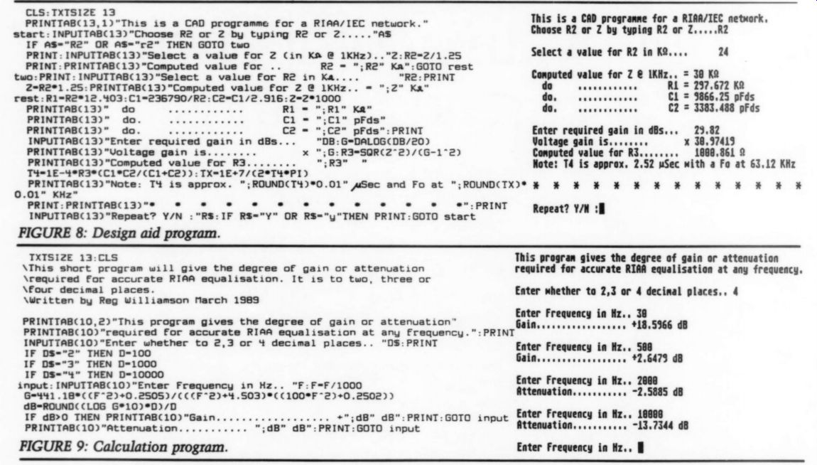
FIGURE 8: Design aid program.
--------------------
FIGURE 9: Calculation program.
------------------------
It'll then ask you what gain you require in dBs. Now, here is the tricky bit.
You must consider the likely peak output of your cartridge, take into ac count the gain you are asking for and then decide, is there likelihood of over load of the active element-the amplifier stage (which could be an op amp or a discrete circuit)? Then there is another factor involved, that is often overlooked --the possibility of it running out of feedback at some point high in the spectrum. This arises because of another time constant, that of R3 and all the reactive elements in Z,,. This is T4 and it will always be there. But as long as it is well above 20kHz, it won't matter much. If it does worry you, then take care of it with a simple passive network at the output, like the one in Fig. 3.
The program calculates T4 for you, along with a value for R3. And that's it.
The main virtue of the CAD program is that you can readjust parameters to your heart's content, until you find nice off-the-peg values and the gain you want. One oddity I discovered is that by using Fig. 5(b) it seemed much easier to find C and R values close to those you can get in the preferred value ranges. I'm including another short program (Fig. 9), written out of sheer laziness, since it proved tiresome to keep entering the complex formula into my calculator when plotting the curve. It computes loss/gain values for any point in the RIAA curve and up to three decimal places, if you wish. Again, you can translate it to any other version of BASIC with little trouble.
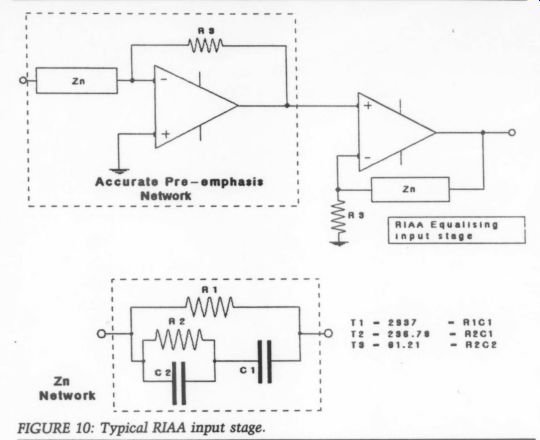
Fig. 10
An Addendum
Since writing this article, I have been fortunate enough to access a sophisticated analyzer program at the University of Keele, England, which allows you to input quite complex linear electronic circuits, with all the important parameters of a wide range of active and passive components. It then produces a highly accurate analysis of how the circuit will behave, tabulating all important parameters in both numerical and graphic form. These include frequency response, phase shift, group delay and input/output impedance.
As an interesting exercise, I simulated an RIAA pre-emphasis equalizer with a high degree of accuracy, then input the equalized signal to a typical RIAA input stage of the type I have been describing.
GRAPH 2: Overall bandwidth deviation.
GRAPH 3: Deviation after T4 correction.
In this case, I did not use the computed values, but off-the-shelf 1% components. As you will see, if you wish for a gain of say, 28.82 dB, then R3 computes to 1k, R1 is 297.672k, R2 is 24k, C1is 9,866.25pF and C2 is 3,383.488 pF.
The op amp is the ubiquitous TL01.
So I substituted an off-the-peg 300k for R1, C1 became 10nF and I selected C2 as 3,600pF. I normalized the insertion loss of the pre-equalization stage to complement the computed gain of 29.82dB of the post-equalization stage, so the overall would be 0dB.
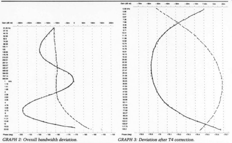
After a simulation run, the results were quite fascinating, showing a negligible midband error of -0.12dB. But it was over the whole band, from 32.25Hz to 22.63kHz, that the results proved most educational. A passband deviation of 0.14dB was apparent, or in communications engineer's parlance, a “spread” of 0.28dB. This, I must suggest again, is so small compared with the typical spread of all transducers in the audio chain, that it may be safely discounted.
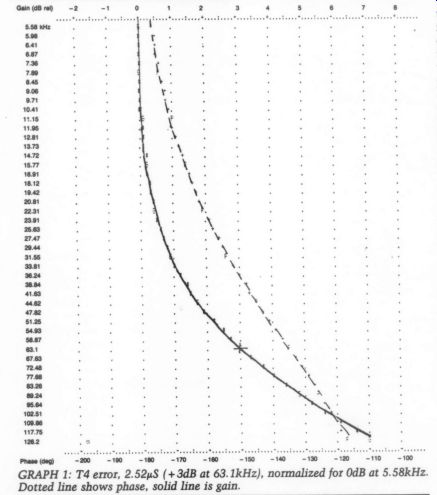
It also showed the effect of T4 quite clearly by the phase shift (dotted line) and the gain rise at the high end. You may correct this with a simple first order filter configuration. Graph 2 shows the overall band error and Graph 3 the corrected T4 error; both are scaled in milli-decibels (0.001dB). The T4 error in Graph 1 is scaled in decibels. Dotted lines indicate phase shift which is so small, it may be discounted.
++++++++++++++
Also see: