AMAZON multi-meters discounts AMAZON oscilloscope discounts
The cathode-ray oscilloscope (CRO) (FIG. 1) is a device that is capable of writing a two-dimensional (2D) and, in some cases, a three-dimensional (3D) graph on a glass screen. It does this under the influence of two (or three)
input signals whose effect is to produce a recognizable pattern that describes certain features of the various signals. At this point you should revise these topics in Sections 11 and 12 (Level-2 Book). Oscilloscopes are the mainstay of circuit testing because circuits are usually designed to operate on signals that change with time and very few, apart from power supplies, are designed not to change with time.
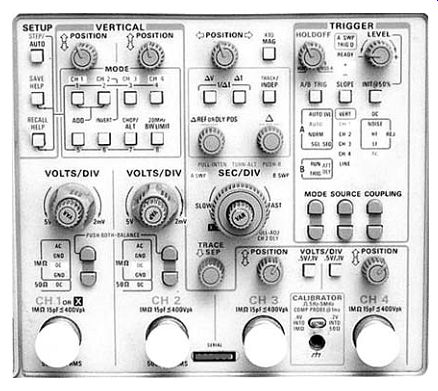
FIG. 1. A typical analog oscilloscope, the Tektronix 202445A
The older type of oscilloscope is purely analog in nature and to over come the transient nature of the display, the CRO can be fitted with a camera attachment to provide a permanent record. Each oscilloscope type is commonly available with a range of alternate cathode-ray tubes (CRTs), each with a different persistence of illumination and color.
At the heart of the display system is the sawtooth waveform that is used to produce the horizontal beam deflection across the tube face. This causes the beam to traverse the screen relatively slowly during the forward writing period and then rapidly fly back to repeat the process in a continuous manner. While this is in progress, the signal to be examined, the work signal, is applied to the vertical deflection system so that a 2D pattern that describes its amplitude, periodic time and general shape can be displayed. Typical basic beam-deflection sensitivities, which are accurately known for each tube, vary between 0.02 and 0.05 cm/V.
A CRO with a single-beam CRT can function as a multi-trace CRO in one of two modes, chopped or alternate. In the chopped mode, the beam is rap idly switched many times per trace cycle between two channels to provide a double-trace display. Switching high-frequency signals in this manner produces unacceptable gaps in the displayed waveform and thus this mode is limited to use at relatively low frequencies. In the alternate mode, one sweep is used alternately for each channel, but at the expense of reduced trace brightness. True double-beam CRTs use tubes with two identical electron guns mounted side by side within a common glass envelope. These can also be adapted as above to provide four-channel operation.
Using an analog oscilloscope
The signal to be examined is input to the Y-amplifier section through a calibrated step attenuator which commonly provides an input impedance ranging from 1 to 10 M in parallel with a self-capacitance of 10-20 pF. A few specialized instruments use a 50 O input impedance. This stage typically has a rise time of a few tens of nanoseconds (rise time is the time taken for the signal to rise or fall between its 10% and 90% levels). The input band width can easily exceed 100 MHz. Dual-channel CROs will be equipped with two such stages. The major part of the Y channel gain is achieved in the driver and output stages to the Y-plates.
The X-deflection system is driven from a sawtooth generator stage that provides a waveform with very low distortion. This signal is further amplified before being used to drive the X-deflection system. Again, for a dual or double beam instrument there will be two similar display driver stages, but generally driven from one (or possibly two) timebase circuits. The timebase sawtooth can be synchronized to either of the two input signals (Y) selected by a switch, as shown in FIG. 2. Provision is also commonly available to compare the Y input with an external signal and therefore an additional switched input can be provided as shown. In addition, d.c. shift potentials are provided for both the X and Y channels to position the trace precisely within the graticule scale, which is commonly ruled in 1 cm squares.
At times, it is necessary to study just a short time-scale section of the Y signal and this can be done by blanking this input until such times as the important section becomes available. This can then be studied by illuminating the trace through a bright-up signal known as the Z modulation, so that only the wanted period is displayed. The effect is almost that of a 3D display.
The visual display is supported by an engraved and sometimes illuminated measuring scale called a graticule. This allows fairly accurate assessments of amplitude, phase relationship and time to be made. In addition, with experience it is possible to obtain a reasonable assessment of any distortion found in a waveform.
===
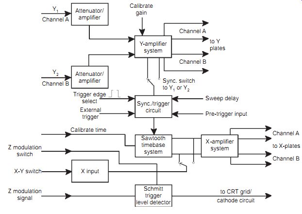
FIG. 2 Block diagram of two-channel analog oscilloscope
====
Normally, the Y input is coupled via a high value of capacitor to ensure that the frequency response can extend as low as 10 Hz. The CRO is equipped with a switch labeled a.c./d.c./ground and in the d.c. position the coupling capacitor is short-circuited. This is provided so that the Y input signal that has a d.c. component can be displayed correctly. The ground position is useful because it sets the unmodulated horizontal trace at ground voltage level, which allows this axis to be accurately positioned on a particular graticule line referenced as zero volts.
Even with relatively low-cost oscilloscopes several variations of the basic synchronism (sync.) system can be provided. The timebase can be synchronized from an external source, from either the rising or falling edges of the Y input, or even a range of input signal levels, to avoid false sync. through noise or glitches. When a second auxiliary timebase is provided, this can be used as a delay to sweep the sync. system through sections of very long waveforms in order to examine short period intervals of interest. Again, in some oscilloscopes pre-triggering is provided so that it is possible to examine part of a waveform that would appear before the normal sync. pulse.
Like all test instruments, it is important to be able to rely on the accuracy of the readings obtained. The CRO usually has a built in calibrator that periodically needs to be checked against some standard. The substandard typically consists of an internally generated square wave with a frequency of 1 kHz and amplitude of 1 V. When used as the working input, the gain of the Y amplifier can be preset to indicate an amplitude of 1 V. The periodic time for this waveform is 1 ms and thus the duration of one timebase scan can be similarly adjusted.
The resistive component of the input impedance will load the d.c. conditions of a circuit, while the capacitive component can distort the signal wave form to be examined. While the total input impedance at the Y sockets can be around 10 M in parallel with 20 pF, this can be seriously compromised by the cable used to connect to the circuit under test. The use of a low-loss coaxial cable that is too long can easily distort the leading and trailing edges of square waves. Even the sine-wave frequency response can be affected because the combination of circuit output resistance and CRO input capacitance can act as an integrator or a low-pass filter.
When the CRO is used to measure pulse waveforms in medium to high resistance circuits, a low-capacitance probe should be used. Such probes are available as extras for most types of oscilloscope. A few probes are active in that they contain transistor or field-effect transistor (FET) amplifiers, but most are passive, containing only a variable capacitor and a resistor, as shown in FIG. 3. The input voltage is divided down, so that a more sensitive voltage range must be selected; but the effect of capacitance is greatly reduced because the capacitance of both the cable and the CRO input is used as part of the divider chain.
===
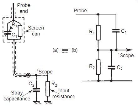
FIG. 3 Passive probe circuit: (a) layout, and (b) equivalent circuit
===
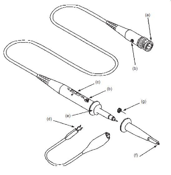
FIG. 4 Oscilloscope probe: (a) BNC connector plugs into probe socket
on oscilloscope front panel, (b) frequency compensation preset, (c) range
switch, (d) ground lead, (e) ground lead connection below finger guard,
(f) probe hook, and (g) spring ground connection
===
Analog oscilloscopes usually require the user to work out the effect of the probe on signal amplitude. For example, if the oscilloscope is on a 1 V per division range with a x10 probe then it is read as 10 V per division. Digital and personal computer (PC)-based instruments usually allow the probe factor to be entered in a menu and then correct all readings to that value.
Be careful with probes that can be set to different ranges using a switch. If the readings seem unreasonable, for example 30 V in a 5 V circuit, the oscilloscope is probably set for x10 probe and the probe is set for x1.
Oscilloscope probes must be matched with the oscilloscope input that they are used with and to this end frequency compensation presets are provided, at one or other end of the probe lead, marked (b) in FIG. 4.
===
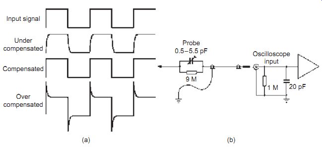
FIG. 5 Oscilloscope probe compensation:
(a) waveforms, and (b) schematic of a x10 passive probe
====
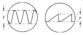
FIG. 6 Measuring peak-to-peak amplitude
===
The compensation matches the resistive divider to the oscilloscope input, which otherwise can look like a low-pass filter. A square-wave test signal with fast rise and fall times is provided on the front panel of the oscilloscope to assist in the adjustment of the compensation preset. Probes should be checked (FIG. 5) using this signal from time to time, and particularly if they have been used with different oscilloscopes, to check that they still match.
Oscilloscope probes are usually of the switchable type, with x1 and x10 ranges and sometimes a reference position selectable on the probe. The reference position grounds the probe circuit locally so that the d.c. level can be adjusted on the oscilloscope display. Most probes isolate the tip when the reference position is selected to avoid dangerous short-circuits.
In the equivalent circuit of the low-capacitance probe (b), C2 includes the stray capacitances of the cable and of the oscilloscope. C1 is varied until R1C1 = R2C2. The signal attenuation which is given by the expression R2/(R1 + R2) shows how it is necessary to select a more sensitive oscilloscope range setting. The probe is normally calibrated against the inbuilt 1 kHz 1 V peak-to-peak (p-p) internal square-wave calibration source.
The basic probe arrangement illustrated here can be extended to provide a x1/x10 input attenuator probe by including a switched resistor network.
Again, this device has to be calibrated in a similar manner to that described above.
To measure the peak-to-peak amplitude of a signal, the vertical distance, in centimeters, between the positive and negative peaks must be taken, using the graticule divisions. This distance (y in FIG. 6) is then multiplied by the figure of sensitivity set on the Volts/cm input sensitivity control.
To measure the duration of a cycle of an a.c. signal, its periodic time, between successive positive or negative peaks, the horizontal distance between them is taken, using the graticule scale (FIG. 7). This distance in centimeters is then multiplied by the time value read off the Time/cm switch scale. The frequency of the wave can be calculated from the formula:
Frequency = 1 /Periodic time
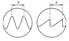
FIG. 7 Measuring the periodic time of waveforms
===
EXPERIMENT 1
Connect a signal generator to the input terminals of the CRO. Set the signal generator so as to provide a 1 kHz square wave of 1 V p-p. Adjust the CRO so as to obtain a locked waveform, and read the amplitude and time. Does the time reading correspond to the frequency as set on the signal generator? Compare these settings with those obtained from the inbuilt calibration signal. Change the signal generator waveform, amplitude and frequency settings, and measure the new waveform's amplitude and periodic time on the CRO. Check that these values agree with the generator settings.
===
With time measured in units of seconds, the calculated frequency will be given by the formula in hertz (Hz). If the time is measured in milliseconds (ms), the frequency will be in units of kilohertz (kHz); if the time is in microseconds (µs), the frequency will be in megahertz (MHz).
To use the CRO to maximum advantage, especially its more sophisticated modes of operation, it is important to obtain as much real-time practice as possible.
An oscilloscope fitted with an external trigger (EXT. TRIG.) input can be used for comparing the phases of two waves if a double-beam CRO is not available. Feeding a signal into the EXT. TRIG. input, with the trigger selector switch set to EXT, will cause the timebase to be triggered by that wave form. The timebase will now always start at the same point in the waveform.
The triggering wave can be seen on the screen by connecting the Y-INPUT socket to the same source. The X and Y shifts can be used to locate one peak of the wave over the centre of the graticule, as illustrated in FIG. 8, which shows one leading edge of a pulse coinciding with the vertical line of the graticule.
Example: A complete cycle of a waveform takes 3 ms, and a second wave has its peak shifted by 0.5 ms. What is the phase difference between the two waves?
Solution: Using the formula above, ? _ (360 _ 0.5)/3 _ 60º.
Now the Y-INPUT from the first waveform is disconnected and replaced by the second source at the same frequency. A locked trace will appear on the screen. If there is a time difference between the two waveforms, the peak of the second wave will not be over the centre of the screen, because the timebase is still being triggered by the first waveform. Measuring the distance X horizontally from the centre allows the calculation of the time shift either earlier (left of centre) or later (right of centre) of the second waveform compared with the first. This time difference can be converted into phase angle if the two waveforms are sine waves. The conversion formula is:
theta=360 x t / T
where ? is the phase angle in degrees, t is the time difference, and T is the time of a complete cycle expressed in the same units as t.
Periodically, both the X and Y amplifier circuits need to be recalibrated.
Carry out this operation using the internal square-wave standard as follows.
Check the bandwidth of the Y amplifier chain by proceeding as follows.
Using a standard sine-wave signal generator, provide an input signal with an amplitude to produce a 5 cm p-p trace. Progressively increase the generator output frequency while maintaining the same input level and note the frequency at which the amplitude falls to 5 x 0.707 = 3.535 cm (approx. 3.5 cm). This is the upper cut-off frequency, and since the Y amplifier must have a d.c. response, it is also the amplifier bandwidth. Check that this figure agrees with that stated in the instrument service manual.
===
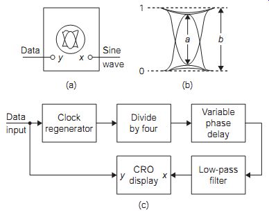
FIG. 9 Producing eye diagrams
===
Digital measurements
Processing a digital signal will create pulse distortion. What starts as a train of square pulses rapidly approaches sine waves as the high-frequency components are progressively removed. This can be measured using an eye diagram. The basic principle is shown in FIG. 9(a), where a digital data stream is applied to the CRO Y input. A sinusoidal timebase is provided at the external X input, running at a quarter of the bit rate.
When the phasing of the two inputs is correctly adjusted, an eye pattern appears as indicated in FIG. 9(b). The upper and lower levels of this trace, which represent the levels produced by a run of several consecutive 1 s and 0 s in the data stream, are taken as the maximum eye opening. A large amplitude of eye opening represents a low level of data distortion and hence a low bit error rate (BER). The ratio of (a/b) x 100% can therefore be used to evaluate the quality of the data signal at various points in the signal processing chain.
FIG. 9(c) shows the classical way in which an eye height display can be produced. The original data stream is used first to lock a local clock oscillator circuit to the bit rate. This is then divided by four and low-pass filtered to provide the one-quarter rate timebase frequency. The data and sinusoid are then input to the CRO as described above. An eye pattern will be displayed when the variable phase delay is correctly adjusted.
Storage oscilloscopes
Storage oscilloscopes are used to display fast, one-shot, transient events or very low frequencies that change too slowly to be captured by the normal persistence CRO tubes. These instruments are available in either digital or analog form, but the analog form is by now obsolete. In the digital form, the signal of interest is first captured, then digitized and stored in a semiconductor memory. From here it is readily available for future display and analysis.
FIG. 10 shows the basic principles of the operation of a digital storage oscilloscope (DSO). The work signal or Y input stages are very similar in circuitry and function to those found in the conventional CRO. High input impedance, high bandwidth and fast rise time are typical of those parameters found in the best of analog instruments. This input stage carries the familiar calibrated attenuator, together with buffer amplifiers to avoid loading the driving circuits under investigation. This stage is followed by analog-to-digital signal conversion before the data is stored in a semi conductor signal acquisition memory, all under the control of the software stored in the control microprocessor. The processed data is then passed through the microprocessor bus system to the display memory, where it is organized into a high speed raster scan format for readout and then display on a CRT or liquid crystal display (LCD) screen.
The display data can be stored in a disk memory (either hard or floppy drive) for future replay and investigation. It is also possible to obtain a hard-copy printout via a standard printer port.
An advantage of digital oscilloscopes is their ability to measure the input signal characteristics directly, for instance peak-to-peak voltage or frequency. FIG. 11 shows a screen capture from a digital oscilloscope (TDS3200) in which the measurements and settings of the channels are clearly displayed.
Both the analog and digital CROs still have their place within the servicing environment because each type has advantages that are not found in the other. The analog real-time (ART) instruments have been in use for a long time and their operation and use are thus very well understood. Because the display is in real time, any fleeting signals become very difficult to capture by any recording method, other than a camera. This in itself would create film processing problems if the Polaroid Land camera had not been developed for this purpose. Even with this it is still very difficult to synchronize and photograph a very brief fleeting signal feature unless it is in some way repetitive. The DSO can display and store slow waveforms and short duration transients with equal ease. It also has the ability to store the waveform data and rerun it on demand. The DSO can perform watchdog facilities such as searching for a glitch or other fleeting signal feature over a long period, plus providing multichannel operation, with automated measurement facilities.
The ART provides waveform information that is truly real time, while the DSO outputs are delayed somewhat owing to signal processing.
===
A to D converter Signal acquisition memory Control micro processor Printer Disk drive (hard or floppy) Display memory CRO/LCD display y Input Attenuator / amplifier
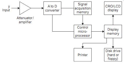
FIG. 10 Block diagram of a digital storage oscilloscope
===
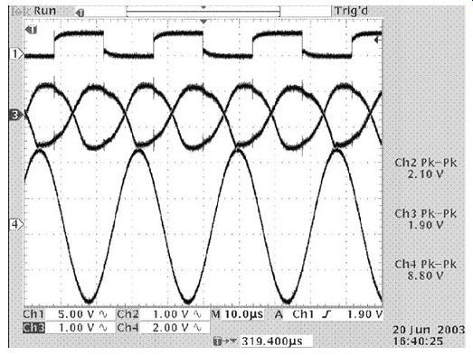
FIG. 11 Typical oscilloscope display, showing channel amplitude settings
and measurements
====
EXPERIMENT 2
Use digital oscilloscopes (a) in real-time mode, and (b) in storage mode. A PC virtual oscilloscope can be used if dedicated hardware is not available.
===
The input signal must be sampled at a rate at least twice that of its highest frequency component to avoid aliasing, which creates distortion and introduces additional frequencies into the waveform. The quantization rate must be at least 8 bits and preferably 12 bits per sample. For example, if the DSO has a response extending from d.c. to 500 MHz, then the sampling rate must be at least 1 GS/s (giga samples per second). At 10 bits per sample this represents a bit rate of 10 Gbit/s. Because of these features, the DSO has a greater accuracy for both the Y system and the X timebase.
A complex signal with many components, such as that found in television systems, is not always easy to resolve using either an ART or a DSO.
Because of the extensive add-ons that have been introduced into both systems over time, it has become rather difficult to learn how to manage such instruments effectively with a wide range of features. Practice therefore is particularly important.
By the very nature of the instrument, the CRO carries a great deal of information about its serviceability within its display. Hence, by observation of the screen display, many of the typical faults may be localized to one of three separate areas:
• faults that affect the CRT and the power supplies
• faults associated with the X input and timebase stages
• faults in the Y amplifier stages that affect the work signal being displayed.
Individual faults can then be located using a second CRO.
The procedure for replacing a faulty or damaged tube varies somewhat from one oscilloscope to another, and the manufacturer's handbook should always be consulted. The glassware is most vulnerable at the tube neck and base connector where the glass changes shape most rapidly. The following general notes will nevertheless be useful.
1. Always wear safety goggles and gloves to avoid injury from flying glass; there is a the risk of implosion.
2. Cover the workbench surface with a blanket or similar material. Place the CRO on a clean bench, with sufficient space available to lay the CRT alongside it once it has been removed.
3. Disconnect the instrument from the power supply, and discharge all capacitors. Any outer coating of carbon on the tube should be treated with respect; it may have acquired a significant charge which needs to be earthed for safety.
4. Remove carefully the tube base, the high-voltage connectors and the leads to the deflection system. For a circular tube it will be necessary to note the particular alignment in respect of the deflection connectors.
5. Carefully remove the tube clamps and screens. Lift the tube out carefully to protect it from any impact. Place the tube on the blanket so that it can not roll off on to the floor (circular tubes only).
6. Observe all safety precautions until the displaced tube is safely packed into its crate for disposal and then complete the reassembly of the CRO.
7. Finally, test and recalibrate.
QUIZ:
1. The graph, right, shows a waveform on the screen of a CRO with the timebase set to 1 ms/cm and the Y attenuator to 1 V/cm. The sawtooth wave is of:
(a) 2 V p-p and 500 Hz frequency
(b) 2 V p-p and 2 kHz frequency
(c) 1 V p-p and 2 kHz frequency
(d) 1 V p-p and 500 Hz frequency.
2. The graph, right, shows the waveforms on the screen of a CRO with the timebase set to 10 ms/cm and the Y attenuator to 5 V/cm. The frequency and peak-to-peak amplitude of waveform A are:
(a) 50 Hz and 10 V
(b) 20 Hz and 20 V
(c) 20 Hz and 10 V
(d) 50 Hz and 20 V.
3. In the same graph with the same settings, waveform A leads waveform B by:
(a) 20 ms
(b) 270º
(c) 90º
(d) 30 ms.
4. In the same graph with the same settings, the frequency and periodic time of both waveforms are:
(a) 50 ms and 20 Hz
(b) 20 ms and 50 Hz
(c) 20 ms and 20 Hz
(d) 50 ms and 50 Hz.
5. For the waveforms shown, right, if the X timebase is set to 100 µs/cm and the Y attenuator to 5 mV/cm, the frequency and peak-to-peak amplitudes of the waves are:
(a) 400 Hz and 2.5 mV
(b) 2.5 kHz and 12.5 mV
(c) 400 Hz and 12.5 mV
(d) 2.5 kHz and 2.5 mV.
6. In the same graph as in question 30.5, waveform B leads waveform A by:
(a) 100 µs
(b) 400 µs
(c) -135º
(d) 135º.