(source: Electronics World, Aug. 1963)

By JACK E. FRECKER / Applied Research Lab., University of Arizona
PART 2 / Applications of the unit, previously discussed, as a voltmeter calibrator, a frequency-sensitive circuit, oscillator, a capacitance bridge, and as a multivibrator.
LAST month the theory and design of operational amplifiers were discussed and the circuit and construction of a two -amplifier unit were shown. The reader will recall that in the most general usage, shown in Fig. 1A, Gain = Eout /Ein = Zf /Zin. Output impedance was assumed to be negligibly small, input impedance at point A was simply the value of Zin, and the effective impedance from point B to ground was quite low. The output current capability of either amplifier was 3 to 5 ma. max. depending on output voltage.
When using the operational amplifier, the open-loop frequency-response curve in Part 1 should be kept in mind. As a rule of thumb, if the open-loop gain at any particular frequency is reduced by a factor of 100 or more by feedback, less than 1% error in calculated gain will result. In the following discussion it will be assumed that the amplifiers are always carefully zero -adjusted and that no attempt is made to use them beyond their frequency capabilities.
Amplifiers and Calibrator
The simplest application is that of Fig. 1A. This is a good general-purpose d.c. and low-frequency (audio) amplifier.
Fig. 1B illustrates a second class of circuit and makes use of the differential input feature of the amplifier. In this circuit Gain = (Zin + Zf) / Zin. and is noninverting. The input impedance is between 100 megohms and 10,000 megohms, depending on the condition of the 6AU6 tubes.
By making Zin an open circuit and Zf a short circuit in Fig. 1B, the unit becomes a unity -gain amplifier similar to a cathode-follower. It is useful as an isolation device to over 100 kilocycles. Another use of this device is shown in Fig. 1.G. The unity-gain amplifier is used as a coaxial -cable shield driver. As the shield is at the same a.c. voltage as the inner conductor, the effective capacity to ground of the inner conductor is reduced nearly to zero. The 1000-ohm resistor is employed in order to prevent parasitic oscillations.
Fig. 1D is the circuit of a voltmeter calibrator. With the switch in the ground position the amplifier is carefully adjusted for zero volts out. Then the switch is turned to the mercury cell and the output voltage, Eout = 1.35 x (Zin + Zf)/ Zin with a very high degree of accuracy.
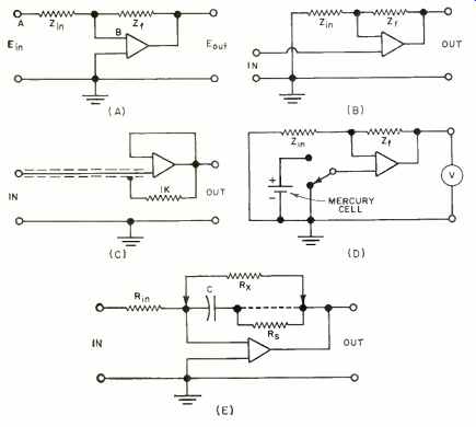
Fig. 1. (A) Basic general-purpose d.c. and low-frequency amplifier. (B)
Isolating amplifier. (C) Coax cable shield driver. (D) Voltmeter calibrator.
(E) Integrator-circuit arrangement.
Integrators
Fig 1E is an integrator. This circuit provides a frequency response roll -off of 6 db per octave. To use this circuit, select the frequency at which gain is to be unity and let X. at this frequency. Then at one-half this frequency the gain will be two, at one -hundredth this frequency the gain will be 100, and so on. R. is necessary to provide some d.c. feedback to prevent the amplifier from drifting into its limits. It should he no larger than 1000Rin. It may be less and, if so, will determine the maximum gain of the amplifier at low frequencies. Also, a resistor can be inserted in series with C. This resistor will determine the minimum gain of the circuit.
With both present the circuit will have a frequency response as shown in Fig. 3A. Fig. 3B is a double integrator. This circuit has a roll off of 12 db per octave. Select the frequency at which the gain is to he one-fourth and let = R at this frequency. Then at one-half this frequency the gain will be unity, at one twentieth this frequency the gain will be 100 and so on.
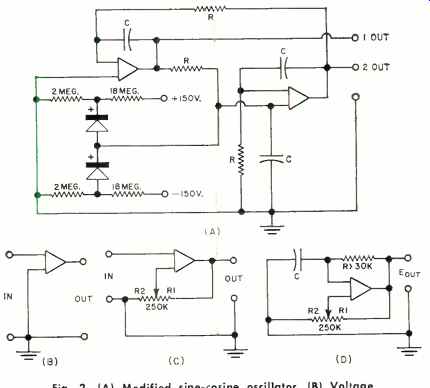
Fig. 2. (A) Modified sine-cosine oscillator. (B) Voltage comparator. (C)
Circuit which adds hysteresis to transfer function. (D) One type of free-running
multivibrator.
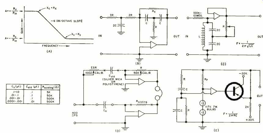
Fig. 3. (A) Frequency response of the circuit shown in Fig. 1E. (B) Double
integrator circuit. (C) "Q "multiplier circuit. (D) Use of operational
amplifier as a capacitance bridge. (E) Wien bridge oscillator connected
to emitter-follower stage.
"Q "Multiplier and Bridge
Fig. 3C is a "Q "multiplier. The unity -gain amplifier output is fed back into the tuned circuit in a regenerative fashion. The effective "Q" of the circuit can be raised by a factor of 50 or more with good stability, and R can be decreased to a point where "Q" becomes infinite and oscillations take place. This circuit is useful to 100 kilocycles but is at its best when it is used within the audio -frequency range.
One of the most potentially useful circuits is the application as a capacitance or resistance bridge. The capacitance bridge is shown in Fig. 3D. In this circuit a low -level audio signal is connected to the input, the capacitor to be measured is connected at C, the appropriate values of C_std, and R are selected and the controls R and ESR are adjusted for a null in the earphones. Frequency is kept low in order that the amplifier open-loop gain will be high and the reactance of Cx and C_std will be high.
The most important advantage, to the experimenter, of this bridge over the completely passive bridge is that the bridge equations are an extremely simple matter of ratio and proportion rather than the gross and involved equations of the conventional types. If perfect components are used, the bridge can measure to an accuracy of .5 per -cent or better. When the bridge is adjusted for a null, C= (R x C_std). Since there are four different combinations of R and C_std, they represent four different multipliers in decade steps.
Equivalent series resistance of C = (ESR x C_std) /C,. Dissipation factor then equals 100R /X. or 200 pi f RC in percent with f in cps, R in ohms, and C in farads. An entire plug -in subassembly unit containing components, switching functions, and a transistor audio oscillator could be constructed along these particular lines.
Sine-Wave Oscillators
Several types of sine-wave oscillators are possible with this unit. The Wien bridge, shown in Fig. 3E is one of the best. The emitter-follower is necessary in this circuit to supply the large amount of driving power required for the bridge. Frequency can be made continuously variable by varying either R or C. R should be always greater than 5000 ohms. Rr is selected to give an output of 7 volts r.m.s.
Another oscillator is a modified form of the sine-cosine oscillator used frequently in analog computer laboratories, and shown in Fig. 2A. The name comes from the fact that there is a 90-degree phase difference between the two outputs. Oscillations build up very slowly in this device and, when they are greater than sixty volts peak-to-peak, a weak diode limiting action takes place tending to hold the amplitude constant.
In the left-hand portion of the circuit, the output leads the input by 90 degrees at all frequencies. The right -hand portion is a noninverting integrator and its output leads its input by 270 degrees. The total of 360 degrees phase shifted signal is fed back to the left-hand unit, and oscillations take place just lower in frequency than where loop gain exceeds unity. This circuit is particularly useful at frequencies from 0.1 cps to 1000 cps. To cause the unit to start faster, momentarily connect + 150 volts to any input through a 10-megohm resistor. All values of R and C should be equal.
Typically, R has a value of 200,000 ohms to 10 megohms.
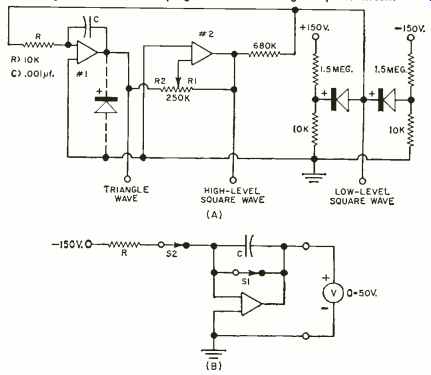
Fig. 4. (A) Waveshaping circuit. (B) Timing computer circuit.
Non-Linear Operation
These amplifiers perform well in nonlinear and limit-to-limit operation if not too much is expected in the way of high frequency performance. A few basic functions will be shown here. The first is a voltage comparator, shown in Fig. 2B. When the input goes ever so slightly positive, the output goes into its negative limit, and vice versa. By connecting the secondary input to some reference voltage, when the input exceeds the reference voltage, the output will go into its negative limit, and vice versa.
Fig. 2C adds hysteresis to the transfer unction. Now the input must exceed a value determined by the output voltage, R1, and R2 to cause the amplifier to S to its negative limit, and then must become less than some more negative new value to cause the amplifier to S into its positive limit.
Fig. 2D is one type of free-running multivibrator using the above principles.
The circuit starts out in one of its limits, but the voltage at C, being charged through R, eventually becomes great enough to cause the amplifier to switch to its other limit. Then C is charged through R in the opposite direction and the amplifier eventually switches back to the first condition described above and so on.
Waveform Generators
Fig. 4A is a highly refined circuit that simultaneously generates square waves and triangular waves with perfectly straight ramps of equal positive and negative slopes. The output of an integrator with a d.c. input, Eia, is a perfectly linear ramp whose slope in volts-per-second equals Eia /RC. In Fig. 4A, when the positive -going voltage out of amplifier No. 1 reaches some value determined by the setting of R1R2, amplifier No. 2 will switch to its positive limit. This output is clipped to plus 1 volt by diode action. This voltage is reapplied to the integrator, amplifier No. 1, and causes its output to decrease linearly to a new value. This causes amplifier No. 2 to switch to its negative limit. This, in turn, causes the integrator to produce a positive-going ramp, and so on.
The slope of the integrator in volts per second with the ± 1 volt clipping action of the diodes is 1/RC. The amplitude and frequency of the triangular wave output are both affected by the setting of R1-R2. This circuit has been used successfully from 1 cycle-per-minute to 1000 cycles-per-second. Typically, R1/ R2 will be from 4:1 to 20:1.
By putting a diode in parallel with R, the waveform is changed from a triangle to a saw-tooth with the fast rise or fast fall determined by the polarity of the diode. Connecting a diode directly from the output of the integrator to ground, as shown, makes the device monostable, and it can be triggered by capacitively coupling a negative voltage spike into the secondary input of amplifier No. 2. This arrangement then makes a device capable of providing a perfectly linear slow triggered sweep for inexpensive oscilloscopes. The high-level square wave is then used to provide retrace blanking for the scope. Obviously, the above waveforms must be direct-coupled to the oscilloscope vertical-input terminals.
Timing Computer
In the foregoing section it was mentioned that the output of an integrator with a d.c. input is a perfectly linear ramp voltage whose slope in volts-per-second equals Eia /RC. Because of this an integrator can be used as a timing device, with output voltage being proportional to time. Such an application is shown in Fig. 4B. In operation S1 is opened first. The output voltage, as measured on the meter, then increases from zero at a perfectly linear rate in respect to time. When S2 is opened, the output voltage will hold its last value. Then time, the interval between the opening of S1 and S2, equals (E_out x RC) /150.
It is necessary to carefully zero-adjust the amplifier immediately prior to use. To do this, open S2 first and then S1.
The meter reading should remain at zero volts. If it drifts off, reset the zero adjust control to cause it not to drift off. C must be a low-leakage unit, preferably polystyrene, silver mica, or Mylar. Otherwise the d.c. leakage will cause errors and drift.
This circuit was used to measure the muzzle velocity of a Grossman carbon dioxide pellet pistol. Si and S2 were actually two strips of aluminum foil 1/8-inch wide and 2 inches long mounted on cardboard frames with cellophane tape. They were placed exactly one foot apart. The gun was then placed a few inches from S1, aimed to first break Si and then S2, and fired. The anticipated time interval was about 3 msec. R was chosen as 100,000 ohms and C as 0.15 µf.
After the gun was fired, the meter indicated 22 volts. Time was then calculated to be 2.2 msec. and velocity to be 1/0.0022 or 455 feet-per-second.
Some of the circuits in this article were taken from material supplied by George A. Philbrick Researches Inc., Boston, Massachusetts.