Electronic Test Instruments: Measurement Theory (part 1)

To understand the operation and use of electronic instruments, it's necessary to review some of the electrical theory associated with electronic measurements. Although it's assumed that the reader understands basic electrical principles (voltage, current, Ohm’s law, etc.), these principles are reviewed here with special emphasis on how the theory relates to electronic measurement. With this approach, the theory is tackled u front to lay the groundwork for discussing the use and operation of electronic instruments. Most of the theoretical concepts apply to multiple types of measurements and instruments.

Electrical Quantities

A discussion on electronic measurements must be preceded by a thorough understanding of the parameters to be measured. Appendix A contains a table of electrical parameters, their units of measure, and standard abbreviations. The standard electrical units can be modified by the use of prefixes (milli, kilo, etc.). Our initial concern is with the measurement of voltage and current (with a slight emphasis on voltage); later, we will include other parameters such as capacitance and inductance.

Current (measured in units of amperes and often abbreviated to amps) is the flow of electrical charge (measured in coulombs). The amount of charge is determined by the number of electrons moving past a given point. An electron has a negative charge of 1.602 x 10^-19 coulombs, or equivalently, a coulomb of negative charge consists of 6.242 x 10^18 electrons. The unit of current (the ampere) is defined as the number of coulombs of charge passing a given point in a second (one ampere equals one coulomb per second). The more charge that moves in a given time, the higher the current. Even though current is usually made up of moving electrons, the standard electrical engineering convention is to consider current to be the flow of positive charge. With this definition, the current is considered to be flowing in a direction opposite to the electron flow (since electrons are negatively charged). (Current is also sometimes defined as electron flow, i.e., the current flows opposite to the direction used in this book.)

Voltage (measured in volts), often referred to as electromotive force (EMF) or electrical potential, is the electrical force or pressure that causes the charge to move and the current to flow. Voltage is a relative concept, i.e., voltage at a given point must be specified relative to some other point, which may be the system common or ground point.

An often used analogy to electrical current is a water pipe with water flowing through it (Figure 1-1). The individual water molecules can be thought of as electrical charge. The amount of water flowing is similar to electrical current. The water pressure (presumably provided by some sort of external pump) corresponds nicely to electrical pressure or voltage. In this case, the water pressure we are interested in is actually the difference between the two pressures at each end of the pipe. If the pressure (voltage) is the same at both ends of the pipe, the water flow (current) is zero. On the other hand, if the pressure (voltage) is higher at one end of the pipe, water (current) flows away from the higher pressure end, to ward the lower pressure end.

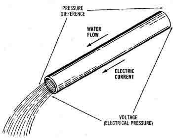
Figure 1-1. The water pipe analogy shows how water flow and pressure difference behave similarly to electrical current and voltage.

Note that while the water flows through the pipe, the water pressure is across the pipe. In the same way, current flows through an electrical device but voltage (electrical pressure) exists across the device (Figure 1-2). This affects the way we connect measuring instruments, depending on whether we are measuring voltage or current. For voltage measurement, the measuring instrument is connected in parallel with the two voltage points (Figure 1-3A). Two points must be specified when refer ring to a particular voltage, and two points are required for a voltage measurement (one of them may be the system ground). Measuring voltage at one point only is incorrect. Often we refer to a voltage at one point when the other point is implied to be the system common or ground point. This is an acceptable practice as long as the assumed second point is made clear.

Current, similar to water flow, passes through a device or circuit. When measuring current, the instrument is inserted into the circuit that we are measuring (Figure 1-3B). (There are some exceptions to this, such as current probes discussed in Section 4.) The circuit is broken at the point the current is to be measured and the instrument is inserted. This results in the current being measured passing through the measuring instrument. To preserve accuracy for both voltage and current measurements, it's important that the measuring instrument not affect the circuit that's being measured.

Resistance

A resistor is an electrical device which obeys Ohm’s law:

I = V/R, or V = IR, or R = V/I

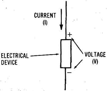
Figure 1-2. Electrical current flows through the device while the voltage exists across the device.

Ohm’s law simply states that the current through a resistor is proportional to the voltage across that resistor. Returning to the water pipe analogy, as the pressure (voltage) is increased, the amount of water flow (current) also increases, If the voltage is reduced, the current is reduced. Carrying the analogy further, the resistance is related inversely to the size of the water pipe. The larger the water pipe, the smaller the resistance to water flow. A large water pipe (small-value resistor) allows a large amount of water (current) to flow for a given pressure (voltage). The name “resistor” is due to the behavior of the device: it resists current. The larger the value of the resistor, the more it resists and the smaller is the current (again, assuming a constant voltage).

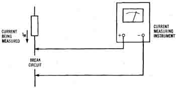
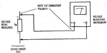
Figure 1-3. Voltage and current measurements.

(A) Voltage measurements are made at two points. Note that the polarity of the measuring instrument is consistent with the polarity of the voltage being measured. (B) Current measurements are made by inserting the measuring instrument into the circuit such that the current flows through the instrument.

Polarity

A small amount of care must be taken to ensure that voltages and currents calculated or measured have the proper direction associated with them. The standard engineering sign convention (definition of the direction of the current relative to the polarity of the voltage) is shown in Figure 1-4. A voltage source (V) is connected to a resistor (R) and some current (I) flows through the resistor. The direction of I is such that for a positive voltage source, a positive current will leave the voltage source at the positive terminal and enter the resistor at its most positive end. (Remember, current is taken to be the flow of positive charge. The electrons would actually be moving opposite the current flow.) Figure 1-3 shows the measuring instrument connected up in a manner consistent with the directions in Figure 1-4.

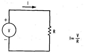
Figure 1-4. Ohm’s law is used to determine the amount of current (I) that will result with voltage (V) and resistance (R).

If the measuring instruments are connected up with the wrong polarity (backwards) when making direct current (DC) measurements, the instrument will attempt to measure the proper value, but with the wrong sign (e.g. -5 volts instead of +5 volts). Typically, in digital instruments this is no problem. A minus sign is just added in front of the reading. In an analog instrument the reading will usually go off the scale and if an electromechanical meter is used it will deflect the meter in the reverse direction, often causing damage. It is best to consult the operating manual to understand the limitations of the particular instrument before attempting measurements. Polarity is most often not a consideration for AC measurements, unless phase is being measured.

EXAMPLE 1-1. Calculate the amount of voltage across a 5- kilo-ohm resistor if 3 mA of current are flowing through it. Using Ohm’s law, V=IR=(.003)(5000) volts

Direct Current

Direct current (DC) is the simplest form of current. Both current and voltage are constant. (Even though the term “DC” specifically states direct current, it's used to describe both voltage and current. This leads to commonly used, but self-contradictory terminology such as “DC voltage” which means, literally, “direct current voltage.”) A plot of DC voltage vs. time is shown in Figure 1-5. This plot should seem rather uninformative, since it shows the same voltage for all values of time, but will contrast well with alternating current when it's introduced.

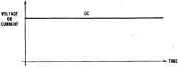
Figure 1-5. DC voltages and currents are constant with respect to time.

Both batteries and DC power supplies produce DC voltage. Batteries are available with quite a variety of voltage and current ratings. DC power supplies convert AC voltages into DC voltages and are discussed in Section 6.

POWER

Power is the rate at which energy flows from one circuit to another circuit. For DC voltages and currents, power is simply the voltage times the current and the unit is the watt:

P=VI

Using Ohm’s Law and some simple math, the relationships in Chart 1-1 can be developed. Notice that power depends on both current and voltage. There can be high voltage but no power if there is no path for the current. Or there could be a large current through a device with zero volts across it, also resulting in no power being received by the device.

Chart 1-1. Basic Equations for DC Voltage, DC Current, Resistance, and Power

Alternating Current

Alternating current (AC), as the name implies, does not remain constant like direct current, but instead changes direction (alternates) at some frequency. The most common form of AC is the sine wave, as shown in Figure 1-6. The current or voltage starts out at zero, becomes positive for one half of the cycle and then passes through zero to become negative for the second half of the cycle. This cycle then repeats continuously. The voltage of the waveform can be described by the RMS value, zero-to-peak value, or the peak-to-peak value.

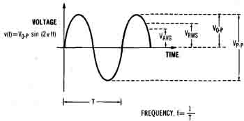
Figure 1-6. The most common form of alternating current is the sine wave.

The length of the cycle (in seconds) is called the period and is represented by the symbol T. The frequency, f, is the reciprocal of the period and is measured in units of hertz, which is equivalent to cycles per second.

f = 1/T

The frequency indicates how many cycles the sine wave completes in one second. For example, the standard AC power line voltage in the U.S. has a frequency of 60 Hz which means that the voltage goes through 60 complete cycles in one second. The period of a 60-liz sine wave is T = 1/f = 1/60 = 0.0167 sec.

Since the sine wave is not constant with time, it's not immediately obvious how to describe its voltage. Sometimes the voltage is positive, sometimes it's negative and twice every cycle it's zero. This problem does not exist with DC, since it's always a constant value. Figure 1-6 shows four different ways of referring to AC voltage. The zero-to-peak value (V0-p) is simply the maximum voltage that the sine wave reaches. Similarly, the peak-to-peak value (Vp-p) is measured from the maximum positive voltage to the most negative voltage. For a sine wave, Vp-p is always twice V0-p.

RMS Value

The third way of referring to AC voltage is the RMS or effective value RMS is an abbreviation for Root-Mean-Square, which indicates the mathematics behind calculating the value of arbitrary waveforms. To calculate the RMS value of a waveform, the waveform is first squared at every point. Then, the average or mean value of this squared waveform is found. Finally, the square root of the mean value is taken to produce the RMS (root of the mean of the square) value. (See Appendix E for a more mathematical description of RMS value.)

Determining the RMS value from the zero-to-peak value (or vice versa) can be difficult due to the complexity of the RMS operation. Fortunately, the relationship has been computed for the sine wave and is very straightforward. This relationship is valid only for a sine wave and does not hold for other waveforms.

Average Value

Finally, voltage is sometimes defined using an average value. Strictly speaking, the average value of a sine wave is zero because the waveform is positive for one half cycle and is negative for the other half. Since the two halves are symmetrical, they cancel out when they are averaged together. So, on the average, the waveform voltage is zero.

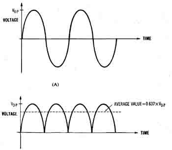
Figure 1-7. The operations involved in finding the fullwave average value of a sine wave. (A) The original sine wave. (B) The full-wave rectified version of the sine wave.

Another interpretation of average value is to assume that the wave form has been full-wave rectified. Mathematically this means that the absolute value of the waveform is used (i.e. the negative portion of the cycle has been treated as being positive). (In a later section we will follow with a more mathematical description of full-wave rectified average value.) This is exactly what some measurement instruments do to handle AC wave forms, so that's what will be considered here. Unless otherwise indicated, Vavg will mean the full-wave rectified average. These averaging steps have been shown in Figure 1-7. Figure 1-7A shows a sine wave that's to be full-wave rectified. Figure 1-7B shows the resulting full- wave rectified sine wave. Whenever the original waveform becomes negative, full-wave rectification changes the sign and converts the voltage into a positive waveform with the same amplitude. Graphically, this can be described as folding the negative half of the waveform up onto the positive half, resulting in a humped sort of waveform. Now the average value can be determined and is plotted in Figure 1-7B. The relationship between Vavg and V depends on the shape of the wave form. For a sine wave:

Vavg = (2/π) Vo = 0.637 Vo-p (sine wave

π = 3.14159 (approximately).

Crest Factor

The ratio of the zero-to-peak value to the RMS value of the waveform is known as the crest factor. Crest factor is a measure of how high the waveform peaks, relative to its RMS value. The crest factor of a wave form is important in some measuring instruments. Waveforms with very high crest factors require the measuring instrument to tolerate very large peak voltages while simultaneously measuring the much smaller RMS value.

Crest Factor = Vo-p/Vrms

The peak-to-average ratio, also known as average crest factor, is similar to crest factor except that the average value of the waveform is used in the denominator of the ratio. It is a measure of how high the peaks of the waveform are compared to its average value.

Although the preceding discussion has referred to AC voltages, the same concepts apply to AC currents. That is, AC currents can be de scribed by their zero-to-peak, peak-to-peak, RMS, and average values.

Phase

The voltage specifies the amplitude or height of the sine wave, and the frequency (or the period) specifies how often the sine wave completes a cycle. But two sine waves of the same frequency may not cross zero at the same time. Therefore, the phase of the sine wave is used to define its position on the time axis. The unit of phase is the degree, with one cycle of a sine wave divided up into 360 degrees of phase. Since there is no universal time when phase equals zero, phase is a relative concept. In other words, we can talk about phase between two sine waves, but not the phase of a single, isolated sine wave (unless some other sort of time reference is supplied).

For example, the two sine waves in Figure 1-8A are separated by one fourth of a cycle (they reach their maximum values one fourth of a cycle apart). Since one cycle equals 360 degrees, the two sine waves have a phase difference of 90 degrees. To be more precise, the second sine wave is 90 degrees behind the first or, equivalently, the second sine wave has a phase of -90 degrees relative to the first sine wave. (The first sine wave has a + 90 degrees phase relative to the second sine wave.) It is also correct to say that the first sine wave leads the second one by 90 degrees, or that the second sine wave lags the first one by 90 degrees. All of these statements specify the same phase relationship.

Figure 1-8B shows two sine waves that are one half cycle (180 degrees) apart. This is the special case where one sine wave is the negative of the other. The phase relationship between two sine waves simply defines how far one sine wave is shifted with respect to the other. When a sine wave is shifted by 360 degrees, it's shifted a complete cycle and is indistinguishable from the original waveform. Because of this, phase is usually specified over a 360 degree range, typically -180 degrees to +180 degrees.

Figure 1-8. The phase of a sine wave defines its relative position on the time axis. (A) The phase between the two sine waves is 90 degrees. (B) The two sine waves are 180 degrees out of phase.

AC Power

The average power dissipated by a resistor with an AC voltage across it's given by:

P = Vrms x Irms = Vrms^2 / R = Irms^2 x R

This relationship holds for any waveform as long as the RMS values of the voltage and current are used. Note that these equations have the same form as the DC case, which is one of the motivations for using RMS values. The RMS value is often called the effective value, since an AC voltage with a given RMS value has the same effect (in terms of power) that a DC voltage with that same value. (A 10-volt RMS AC voltage and a 10-volt DC voltage both supply the same power, 20 watts, to a 5-ohm resistor.) In addition, two AC waveforms that have the same RMS value will cause the same power to be delivered to a resistor. This is NOT true for other voltage descriptions, such as zero-to-peak and peak-to-peak. Thus, RMS is the great equalizer (with respect to power).

EXAMPLE 1-2. The standard line voltage in the U.S. is approximately 115 volts RMS. What are the zero-to-peak, peak-to-peak, and full-wave rectified average voltages? How much power is sup plied to a 200-ohm resistor connected across the line?

Vrms = 0.707 V

thus,

Vo-p = Vpj = 115/0.707 = 162.7 volts

Vp-p = 2 Vo-p= 2 (162.7) = 325.4 volts

Vavg = 0.637 V = 0.637 x 162.7 = 103.6 volts

P = Vrms^2 /R = 115^2/200 = 66.1 watts

Non-sinusoidal Waveforms

There are other AC voltage and current waveforms besides sine waves that are commonly used in electronic systems. Since most of the concepts relating to waveforms apply to both voltage and current waveforms, voltage terminology will be used with the understanding that the same concepts are valid for current waveforms. Voltages are usually, but not always, more easily measured than currents, mainly due to the fact that voltage measurements can be made in parallel with the device being tested without disrupting the circuit paths.

Some of the more common waveforms are shown in Chart 1-2. Note that the values of V and VAVG (relative to V are unique for each waveform. Vavg is the full-wave rectified average value of the wave form. The first three waveforms are symmetrical about the horizontal axis, but the half sine wave and the pulse train are always positive. All of these waveforms are periodic because they repeat the same cycle or period continuously.

An example will help to emphasize the utility of RMS voltages when dealing with power in different waveforms.

EXAMPLE 1-3. A sine wave voltage and a triangle wave voltage are each connected across two separate 300 ohm resistors. If both waveforms deliver 2 watts (average power) to their respective resistors, what are the RMS and zero-to-peak voltages of each waveform?

The two waveforms deliver the same power to identical resistors, so their RMS voltages must be the same. (This is NOT true of their zero-to-peak values.)

P = Vrms^2 / R

Vrms = sqr-rt(PR) = sqr-rt(2(300)) = 24.5 volts RMS

From Chart 1-2, for the sine wave:

Vrms = 0.707 Vo-p

Vo-p = Vrms/0.707 = 24.5/0.707 = 34.7 volts

For the triangle wave:

Vrms = 0.577 Vo-p

Vo-p = Vrms/0.577 = 24.5/0.577 = 42.5 volts

So for the triangle wave to supply the same average power to a resistor, it must reach a higher peak voltage than the sine wave.

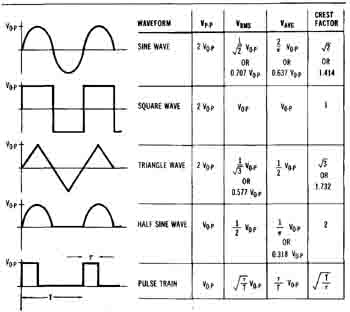
Chart 1-2. Table of Waveforms with Peak-to-Peak Voltage (Vp-p), RMS Voltage (Vrms), Full-Wave Rectified Average Voltage (Vavg), and Crest Factor for Each Waveform

Harmonics

Periodic waveforms, except for absolutely pure sine waves, produce frequencies called harmonics. Harmonic frequencies are integer multiples of the original or fundamental frequency. For example, a non-sinusoidal waveform with a fundamental frequency of 1 kHz would produce harmonics at 2 kHz, 3 kHz, 4 kHz, etc. There can be any number of harmonics, including infinity, but usually there is a practical limitation on how many need be considered. Each harmonic will, in general, have its own unique phase relative to the fundamental.

Harmonics are produced because periodic waveforms, regardless of shape, can be broken down mathematically into a series of sine waves. But this behavior is more than just mathematics. It is as if the physical world regards the sine wave as the purest, most simple sort of waveform with all other periodic waveforms being made up of collections of sine waves. The result is that a periodic waveform (such as a square wave) is exactly equivalent to a series of sine waves.

Square Wave

Consider the square wave shown in Figure 1-9A. Square waves contain the fundamental frequency plus an infinite number of odd harmonics. In. theory, it takes every one of those infinite number of harmonics to create a true square wave. In practice, the fundamental and several harmonics will approximate a square wave. In Figure 1-9B, the fundamental, third harmonic and fifth harmonic are plotted. (Remember, the even harmonics of a square wave are zero.) Note that the amplitude of each higher harmonic is less than the previous one, so the highest harmonics may be small enough to be ignored. When these harmonics are added up, they produce a waveform that resembles a square wave. Figure 1-9C shows the waveform that results from combining just the fundamental and the third harmonic. Already the waveform starts to look somewhat like a square wave. (Well, a least a little bit.) The fundamental plus the third and fifth harmonics is shown in Figure 1-9D. It is a little more like a square wave. Figures 1-9E and 1-9F each add another harmonic to our square wave approximation and each one resembles a square wave more closely than the previous waveform, if all of the infinite number of harmonics were included, the resulting waveform would be a perfect square wave. So the quality of the square wave is limited by the number of harmonics present.

The amplitude of each harmonic must be just the right value for the resulting wave to be a square wave. In addition, the phase relationships between the harmonics must also be correct. If the harmonics are delayed in time by unequal amounts, the square wave will take on a distorted look even though the amplitudes of the harmonics may be correct. This phenomenon is used to advantage in square-wave testing of amplifiers as discussed in Section 5. It is theoretically possible to electronically construct a square wave by connecting a large number of sine wave generators together such that each one contributes the fundamental frequency or a harmonic with just the right amplitude. In practice, this may be difficult because the frequency and phase of each oscillator must also be precisely controlled.

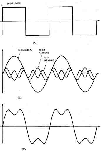
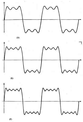
Figure 1-9. The square wave can be broken up into an infinite number of odd harmonics.: (A) The original square wave. (B) The fundamental, third harmonic, and fifth harmonic. (C) The fundamental plus the third harmonic. (D) The fundamental plus the third and fifth harmonics. (E) The fundamental plus the third, fifth, and seventh harmonics. (F) The fundamental plus the third, fifth, seventh, and ninth harmonics.

So far, waveforms have been characterized using a voltage (or cur rent) vs. time plot, which is known as the time domain representation. Another way of describing the same waveform is with frequency on the horizontal axis and voltage on the vertical axis. This is known as the frequency domain representation or spectrum of the waveform. In the frequency domain representation, a vertical line (called a spectral line) indicates a particular frequency that's present (the fundamental or a harmonic). The height of each spectral line corresponds to the amplitude of that particular harmonic. A pure sine wave would be represented by one single spectral line. Figure 1-10 shows the frequency domain representation of a square wave. Notice that only the fundamental and odd harmonics are present and that each harmonic is smaller than the previous one. Understanding the spectral content of waveforms is important because the measurement instrument must be capable of operating at the frequencies of the harmonics (at least the ones that are to be included in the measurement).

Pulse Train

The pulse train, or repetitive pulse, is a common signal in digital systems (Figure 1-11). It is similar to the square wave, but does not have both positive and negative values. Instead it has two possible values: Vo and 0 volts. The square wave spends 50 percent of the time at its positive voltage and 50 percent of the time at its negative voltage. This is referred to as a 50 percent duty cycle. The pulse train’s duty cycle may be any value between 0 and 100 percent and is calculated by the following equation:

Duty Cycle = τ/T

where

τ (tau) is the length of time that the waveform is high

T is the period of the waveform.

Figure 1-10. The frequency domain representation of a square wave, shown out to the 7th harmonic.

The pulse train generates harmonic frequencies with amplitudes that are dependent on the duty cycle. A frequency domain plot of a typical pulse train (duty cycle 25 percent) is shown in Figure 1-12. The envelope of the harmonics has a distinct humped shape which equals zero at integer multiples of hr. Most of the waveform’s energy is contained in the harmonics falling below this hr point. Therefore, it's often used as a rule of thumb for the highest frequency that must be considered in the frequency domain representation.

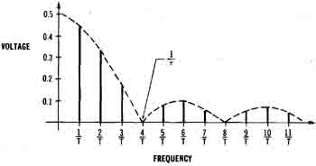
Figure 1-11. The pulse train is a common waveform in digital systems. The duty cycle describes the percent of the time that the waveform is at the higher voltage.

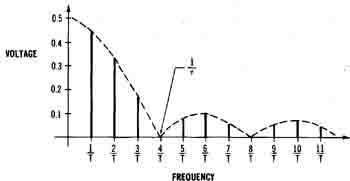
Figure 1-12. The frequency domain plot for a pulse train with a 25% duty cycle.

Table 1-1 summarizes the harmonic content for each of the various waveforms, with V = 1 volt. In all of the waveforms, (except the sine wave) there are an infinite number of harmonics but the amplitudes of the harmonics tend to decrease as the harmonic number increases. At some point, the higher harmonics can be ignored for practical systems because they are so small. As a measure of how wide each waveform is in the frequency domain, the last column lists the number of significant harmonics (ones that are at least 10 percent of the fundamental). Notice that the amplitude value of the fundamental frequency component changes depending on the waveform, even though all of the waveforms have Vo-p = 1 volt. The larger the number of significant harmonics, the wider the signal is in the frequency domain. The sine wave, of course, only has one significant harmonic (the fundamental can be considered the “first” harmonic).

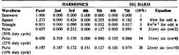
Table 1-1.Table of Harmonics for a Variety of Waveforms

There are two important concepts to be obtained from the previous discussion of harmonics.

1. The more quickly a waveform transitions between its minimum and maximum values, the more significant harmonics it will have and the higher the frequency content of the waveform. For example, the square wave (which has abrupt voltage changes) has more significant harmonics than the triangle wave (which does not change nearly as quickly).

2. The narrower the width of a pulse, the more significant harmonics it will have and the higher the frequency content of the waveform.

Both of these statements should make intuitive sense if one considers that high frequency signals can change voltage faster than lower frequency signals. The two conditions cited above both involve waveforms changing voltage in a more rapid manner. Therefore, it makes sense that waveforms that must change rapidly (those with short rise times and narrow pulses) will have more high frequencies present in the form of harmonics.

EXAMPLE 1-4. What is the highest frequency that must be included in the measurement of a triangle wave that repeats every 50 microseconds (assuming that harmonics less than 10 percent of the fundamental can be ignored)?

The fundamental frequency, f = 1/T = 1/50 microsec = 20 kHz. From Table 1-1, the number of significant harmonics for a triangle wave (using the 10% criterion) is 3. The highest frequency that must be included is 3f = 3(20 kHz) = 60 kHz.

Combined DC and AC

In many cases, the voltage waveform present can be best thought of as being a combination of direct current and alternating current. For example, in transistor circuits, an AC waveform is often superimposed on a DC bias voltage as shown in Figure 1-13. The DC component (a straight horizontal line) and the AC component (a sine wave) combine to form the new waveform.

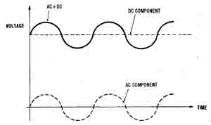
Figure 1-13. The waveform shown can be broken down into a DC component and an AC component.

The DC value of a waveform is also just the waveform’s average value. In Figure 1-13, the waveform is above its DC value half of the time and below the DC value the other half, so on the average the voltage is just the DC value.

Examine the 50 percent duty cycle pulse train shown in Figure 1-14. Notice that the waveform is always positive (never goes below zero volts). The average value is, therefore, greater than zero. The waveform spends half of the time at V and the other half at 0, so the average (DC) value = (Vo-p + 0)/2 = 1/2 Vo-p. The AC component left over when the DC component is removed is a square wave with half the zero-to-peak value of the original pulse train. In summary then, the 50 percent duty cycle pulse train is equivalent to a square wave of half the zero-to-peak voltage plus a 1/2 Vo-p DC component.

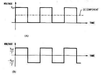Figure 1-14. The 50% duty cycle pulse tram is equivalent to a square wave plus a DC voltage. (A) The pulse train with DC component shown. (B) The square wave that results when the DC component is removed from the pulse train.

EXAMPLE 1-5. A DC power supply has some residual AC riding on top of its DC component, as shown in Figure 1-15. Assuming that the AC component can be measured independently of the DC component, determine both the DC and AC values that would be measured (give the RMS value for the AC component).

The DC value is simply the average value of the waveform. Since the AC component is symmetrical, the average value can be calculated:

DC value = (10.6 + 10.2)/2 = 10.4 volts

If the DC is removed from the waveform, a triangle wave with Vo-p = 0.2 volt is left. For a triangle wave, Vrms = 0.577 Vo-p = 0.115 volt RMS.

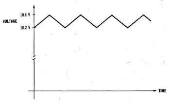
Figure 1-15. DC voltage with a residual triangle wave voltage superimposed on top of it.

Modulated Signals

Sometimes sine waves are modulated by another waveform. For example, communication systems use this technique to superimpose low frequency (voice or data) signals onto a high frequency carrier which can be transmitted long distances. This modulation is performed by modifying some parameter of the original sine wave (called the carrier), depending on the value of the modulating waveform. In this way, information from the modulating waveform is transferred to the carrier. Any characteristic of the carrier can be used. The most common forms of modulation are amplitude, frequency, and phase modulation.

top of page