AMAZON multi-meters discounts AMAZON oscilloscope discounts
Overview
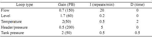
Historically, control functions were originally performed manually by operators (see figure 1). The operator typically used the senses of sight, feel, smell, and sound to "measure the pro cess." To maintain the process within set limits, the operator would adjust a device, such as a manual valve, or change a feed, such as adding a shovelful of coal. The quality of control was poor by today's standards and relied heavily on the capabilities, response, and experience of the human operator.
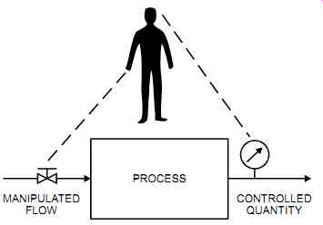
FIG. 1 Typical manual control.
AMAZON multi-meters discounts AMAZON oscilloscope discounts
In modern systems, by contrast, the operator's control function has been replaced by a control unit that continuously compares a measured variable (the feedback) with a set point and automatically produces an output to maintain the process within limits (see FIG. 2). This control unit is the "controller." The operator acts as a supervisor to this controller by setting its set point, which the controller then works to maintain. Automatic controls provide consistent quality products, reduced pollution, labor savings, optimized inventory and production, increased safety, and control of processes that could not be operated manually with any efficiency. In addition, automatic controls release the operator from the need to perform tedious activities, making possible more intelligent and efficient use of labor.
=======
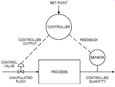
FIG. 2 Typical automatic control.
MANIPULATED FLOW CONTROLLED QUANTITY PROCESS SENSOR FEEDBACK CONTROLLER OUTPUT CONTROL VALVE CONTROLLER SET POINT
=======
Controllers have evolved from simple three-mode pneumatic devices to sophisticated control functions that are part of a larger computer-based system such as a distributed control system (DCS) or a programmable logic controller (PLC). Such microprocessor-based units commonly provide self-tuning, logic control capabilities, digital communication, and so forth.
When selecting a controller for an application, users should keep in mind certain considerations to ensure correct operation. In addition to basic requirements such as the controller's range of input and output signals, accuracy, and speed of response, personnel selecting controllers should also consider
• the effect the controller mode will have on the process if it is left on manual (typically, the transfer from auto mode to manual mode should be a closely controlled activity).
• the ability of the control function to switch bumplessly from automatic to manual and manual to automatic.
• the implementation of direct-reading scales in engineering units.
• the inclusion of built-in external feedback connection (or anti-reset windup) to prevent the development of reset windup caused by the application (refer to the section "Modulating control" later in this Section).
• the effect on the process if the controller fails and the potential need for manual takeover or automatic shutdown.
Control Modes
The two basic modes of control are "on-off" and "modulating." In either case, the values that are the object of measurement are generally referred to as "measured variables" or "process variables" (PV). These variables include chemical composition, flow, level, pressure, and temperature. These measured variables represent the input into the control loop. Before loops can be controlled, the variables must be capable of being measured precisely. The more precisely the variable can be measured, the more precisely the controller controls.
On-Off Control
On-off control (see FIG. 3) is also known as "discrete control" or "two-position" control. In it, the output of the controller changes from one fixed condition to another fixed condition.
Control adjustments are made to the set point and to the differential gap. The differential gap has basically two set points, or one set point with a differential gap or deadband.
On-off control is the simplest and least expensive. It provides some flexibility since the valve size is adjustable. However, it should only be used where cyclic control is permissible (e.g., in large-capacity systems). On-off control cannot provide steady measured values, but it is good enough for many applications.
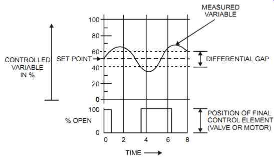
FIG. 3 On-off control.
Modulating Control
In modulating control, the feedback controller operates in two steps. First, it computes the error between the measured variable (the process feedback) and the set point. Then it produces an output signal to the control valve to reduce the measured error to zero.
This type of control-operating with continuously changing analog values-includes three basic functions: proportional, integral, and derivative (PID). Most modern controllers include the three PID functions. Loop operation and tuning parameters may activate a single function, a combination of two functions, or a combination of all three functions.
Proportional (P)
This function, also known as "gain," provides an output that is proportional (in linear relation) to the direction and magnitude of the error signal. The larger the gain, the larger the change in the controller output caused by a given error. Some controller vendors use the term gain while others use proportional band to describe a similar function. The relationship between a controller's gain and its proportional band (PB) is as follows:
Integral (I)
This function, also known as "reset," provides an output that is proportional to the time integral of the input. That is, the output continues to change as long as an error exists. In other words, the integral function acts only when the error exists for a period of time.
The integral function is used to gradually eliminate the offset. Loops with low gain only (i.e., no integral function) will provide stable performance but will generate large offsets, and vice versa. The integral function is slower than the proportional function because it must act over a period of time.
One drawback of the integral function is the "integral windup" (or "reset windup"). This occurs when the deviation cannot be eliminated, such as on open loops, and the controller is therefore driven into its extreme output. This condition creates loss of control for a period of:
PB 100 Gain
----------- =
…time, followed by extreme cycling. Implementing protection from such an occurrence is generally necessary and can be built into the controller as an "anti-integral windup." Derivative (D) The derivative function, also known as "rate," provides an output that is proportional to the rate of change (derivative) of error. In other words, the derivative function acts only when the error is changing with time. The derivative speeds up the controller action, compensating for some of the delays in the feedback loop. It is used to provide quick stability to sudden upsets.
PID Control
When combining the effects of P, I, and D, the typical PID equation is as follows:
where:
Output = controller output Ti
= integral time in minutes
t = time Td
= derivative time in minutes e = error = measured variable - set point (for direct acting controllers)
= set point - measured variable (for reverse acting controllers)
Controller action is available either as direct or reverse. Direct action means that when the measured variable (also known as process variable PV) increases, the output increases.
Reverse action means that when the measured variable increases, the output decreases.
Tuning controllers means setting the values of the PID for optimum performance. Additional information on PID tuning is provided in the section "Controller Tuning" later in this Section.
The following general rules provide an idea of the PID requirements for different loops. How ever, keep in mind that each application has its own needs.
• Flow control: P and I are required; D is set at 0 or at minimum.
• Level control: P is required, I is sometimes required, and D is set at 0 or at minimum.
• Pressure control: P and I are required; D is generally set at 0 or at minimum.
• Temperature control: P, I, and D are required, and the integral action is sometimes fairly long.
Control Types
Four main types of control are commonly used: feedback, cascade, ratio, and feedforward.
Feedback
This is the basic closed loop (see FIG. 4), the oldest type of control. It was developed in 1774 when, in the first industrial application, James Watt used a flyball governor to control the speed of a steam engine.
In a closed loop, a process variable (also know as the "measured variable" or "feedback") is fed as an input into a controller. That input is compared to a set point, and if there is a difference between the two (i.e., an error), the controller output will change in an attempt to bring this error to zero. This output change typically modulates by opening or closing a controlling device, such as a modulating control valve.
An open loop has no feedback and cannot be considered a closed loop. Remember that the operator, who monitors the controlled variable and manually adjusts the output to the valve, acts as a "controller," thereby closing the loop (see FIG. 1). However, the "closing of the loop", by the operator's actions, is not an automatic function, and it totally depends on the operator's sensory capabilities, knowledge, and manual output.
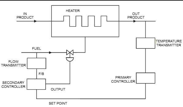
FIG. 4 Typical feedback loop.
Cascade
In cascade control (see FIG. 5), the "primary" variable is controlled by the primary controller (sometimes known as the master), however, it is not a direct control. Instead, it manipulates the set point of the secondary controller, which controls the secondary variable.
Cascade control corrects the disturbances in the secondary loop before they affect the primary process variable. It should be noted that cascade control systems control both primary and secondary variables. To maintain stability, the secondary loop must be much faster than the primary loop, and the secondary loop must receive the maximum disturbances (instead of-and before they affect-the primary loop).
Ratio
In ratio control (see FIG. 6), the controlled variable follows in proportion to a second vari able known as the "wild" variable. The proportionality constant is the ratio. Ratio systems are not limited to two components; one wild flow can adjust several controlled flows.
Feedforward
A feedforward control system (see FIG. 7) measures a disturbance, predicts its effect on the process, and immediately applies corrective action. Feedforward control is by itself insufficient. It is generally used in conjunction with feedback control to trim the feedforward model.
It should be noted that:
• feedforward on its own is an open loop.
• feedforward and feedback systems independently adjust the control valve.
• there is no control applied to the feedforward variable.
============
FIG. 5 Typical cascade loop.
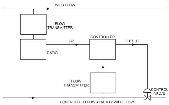
FIG. 6 Typical ratio loop.
=============
Controller Tuning
The performance of a PID control loop depends on the following:
• The quality of the measuring and control devices.
• The effect of process upsets.
• The control stability as manifested in the ability of the measured variable to return to its set point after a disturbance (see FIG. 8). This ability is dependent on the correct controller PID settings, which is accomplished through good tuning.
Tuning means finding the ideal combination of P, I, and D to provide the optimum performance for the loop under operating conditions. Keep in mind that "ideal control" must be determined for a specific application.
=====
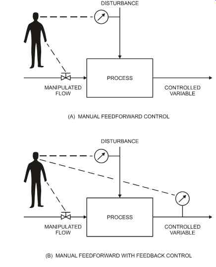
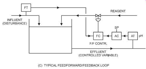
FIG. 7 Feedforward control systems.
=====
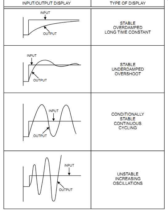
FIG. 8 Typical response curves.
Loops can be tuned either for minimum area, minimum cycling, or minimum deviation (see FIG. 9).
• "Minimum area" produces a longer-lasting deviation from the set point. It is used for applications in which overshoot is detrimental (e.g., a defective product would result).
• "Minimum cycling" produces minimum disturbances with a minimum time duration.
Applications with a number of loops in series benefit from this setup because it provides overall process stability.
• "Minimum deviation" maintains close control with small deviations and is the most commonly used. However, there is cycling around the set point. The amplitude should be kept at minimum.
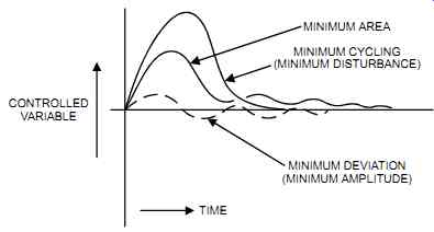
FIG. 9 Different control stabilities.
Controller tuning is generally done automatically, manually, or through adjustments based on experience. In all cases, a few simple rules will minimize problems.
• Check with the operator before starting.
• Before retuning an existing controller, note the old settings (just in case you need to go back to them in a hurry).
• If you are on manual, and the process is steady, take note of the output signal to the valve (in case you need to go back to manual in a hurry).
• On cascade loops, tune the secondary controller first, with its set point in local mode.
Automatic Tuning
In automatic controller tuning, the software/hardware vendor has included a feature in the equipment to perform the tuning function.
Manual Tuning
Manual tuning is a combination of art, science, and experience. In addition, two elements are required for good tuning. First, a good understanding of the loop being tuned is required; second, lots of patience is essential, since some loops may take a long time to properly tune.
There are two basic methods for manual tuning: open loop and closed loop. Open loop tuning may be used to tune loops that have long delays such as analysis and temperature loops, and closed loop tuning may be used to tune fast loops such as flow, pressure, and level loops.
Open Loop
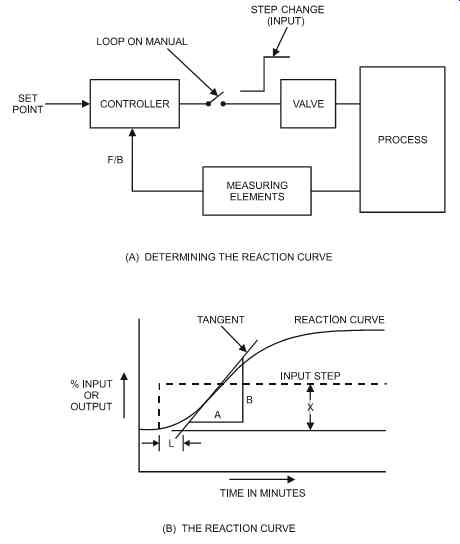
FIG. 10 Open-loop method.
The open loop method (see FIG. 10) consists of the following steps:
• Putting the controller on manual (open loop)
• Making a step change to the output (X) (5 to 10%)
• Recording the resulting action (PV) from the feedback element
• Finding the reaction rate R (= B/A)
• Finding the unit reaction rate Ru (= R/X)
• Finding the effective lag L (time intercept)
• Setting the controller PID values gain = 1.2 / (Ru x L) integral = 0.5 / L in repeats/minute derivative = (0.5) L in minutes
• Where only P and I values are required, the settings are gain = 0.9 / (Ru x L) integral = 0.3 / L in repeats/minute
• Testing and fine tuning, if required
Closed Loop
The Ziegler-Nichols closed loop method (see FIG. 11) consists of the following steps:
• Putting the process on auto control using "P only" mode (set I and D to minimum)
• Moving the controller set point 10 percent and holding until PV begins to move
• Returning the set point to its original value
• Adjusting gain until a stable continuous cycle is obtained (i.e., critical gain, Gc)
• Measuring period of cycle (Pc)
• Setting the controller PID values gain = (0.6) Gc integral = 2 / Pc in repeats/minute derivative = (0.125) Pc in minutes
• Where only P and I values are required, the settings are gain = (0.45) Gc integral = 1.2 / Pc in repeats/minute
• Testing and fine tuning, if required
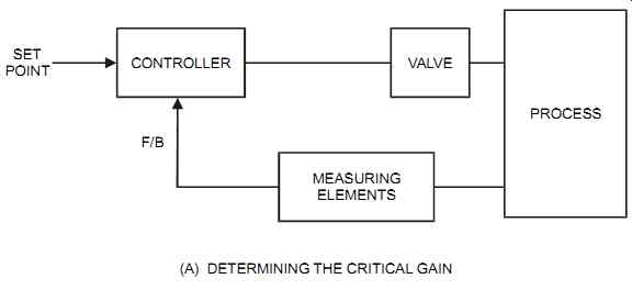
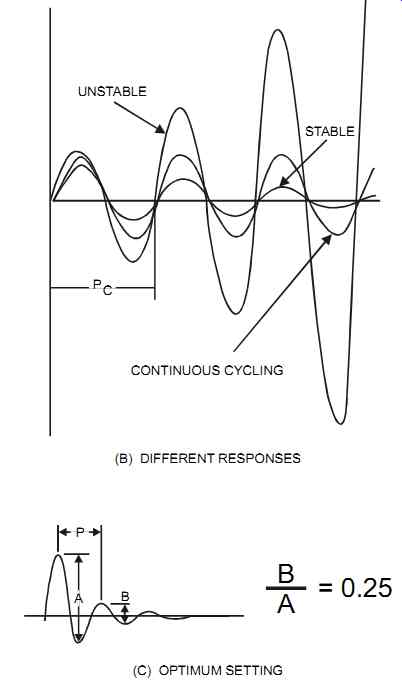
FIG. 11 Closed-loop method. (A) DETERMINING THE CRITICAL GAIN (B) DIFFERENT
RESPONSES (C) OPTIMUM SETTING
Based-on-Experience Tuning
In the tuning method "based-on-experience", known values of P, I, and D are entered. This is a rough way of doing controller tuning, and it does not generally work from the first trial. To make it work, repeated "fine tuning" is required: tweaking the PID settings until acceptable settings are obtained through trial-and-error adjustments. Approximate typical settings for based-on-experience tuning are as follows: