AMAZON multi-meters discounts AMAZON oscilloscope discounts
1. INTRODUCTION
The physical quantity under measurement makes its first contact in the time of measurement with a sensor. A sensor is a device that measures a physical quantity and converts it into a signal which can be read by an observer or by an instrument. For example, a mercury thermometer converts the measured temperature into expansion and contraction of a liquid which can be read on a calibrated glass tube. A thermocouple converts temperature to an output voltage which can be read by a voltmeter. For accuracy, all sensors need to be calibrated against known standards.
In everyday life, sensors are used everywhere such as touch sensitive mobile phones, laptop's touch pad, touch controller light, etc. People use so many applications of sensors in their everyday lifestyle that even they are not aware about it. Examples of such applications are in the field of medicine, machines, cars, aerospace, robotics and manufacturing plants. The sensitivity of the sensors is the change of sensor's output when the measured quantity changes. For example, the output increases 1 volt when the temperature in the thermocouple junction increases 1°C. The sensitivity of the thermocouple element is 1 volt/°C. To measure very small charges, the sensors should have very high sensitivity.
A transducer is a device, usually electrical, electronic, electro-mechanical, electromagnetic, photonic, or photovoltaic that converts one type of energy or physical attribute to another (generally electrical or mechanical) for various measurement purposes including measurement or information transfer (for example, pressure sensors).
The term transducer is commonly used in two senses; the sensor, used to detect a parameter in one form and report it in another (usually an electrical or digital signal), and the audio loudspeaker, which converts electrical voltage variations representing music or speech to mechanical cone vibration and hence vibrates air molecules creating sound.
2. ELECTRICAL TRANSDUCERS
Electrical transducers are defined as the transducers which convert one form of energy to electrical energy for measurement purposes. The quantities which cannot be measured directly, such as pressure, displacement, temperature, humidity, fluid flow, etc., are required to be sensed and changed into electrical signal first for easy measurement.
The advantages of electrical transducers are the following:
• Power requirement is very low for controlling the electrical or electronic system.
• An amplifier may be used for amplifying the electrical signal according to the requirement.
• Friction effect is minimized.
• Mass-inertia effect are also minimized, because in case of electrical or electronics signals the inertia effect is due to the mass of the electrons, which can be negligible.
• The output can be indicated and recorded remotely from the sensing element.
Basic Requirements of a Transducer
The main objective of a transducer is to react only for the measurement under specified limits for which it is designed. It is, therefore, necessary to know the relationship between the input and output quantities and it should be fixed. A transducer should have the following basic requirements:
1. Linearity
Its input vs output characteristics should be linear and it should produce these characteristics in balanced way.
2. Ruggedness
A transducer should be capable of withstanding overload and some safety arrangements must be provided with it for overload protection.
3. Repeatability
The device should reproduce the same output signal when the same input signal is applied again and again under unchanged environmental conditions, e.g., temperature, pressure, humidity, etc.
4. High Reliability and Stability
The transducer should give minimum error in measurement for temperature variations, vibrations and other various changes in surroundings.
5. High Output Signal Quality
The quality of output signal should be good, i.e., the ratio of the signal to the noise should be high and the amplitude of the output signal should be enough.
6. No Hysteresis
It should not give any hysteresis during measurement while input signal is varied from its low value to high value and vice versa.
7. Residual Reformation
There should not be any deformation on removal of input signal after long period of use.
3. LINEAR VARIABLE DIFFERENTIAL TRANSFORMER (LVDT)
The most widely used inductive transducer to translate the linear motion into electrical signals is the Linear Variable Differential Transformer (LVDT). The basic construction of LVDT is shown in Figure 1. The transformer consists of a single primary winding ' P ' and two secondary windings S 1 and S 2 wound on a cylindrical former. A sinusoidal voltage of amplitude 3 to 15 Volt and frequency 50 to 20000 Hz is used to excite the primary. The two secondaries have equal number of turns and are identically placed on either side of the primary winding.
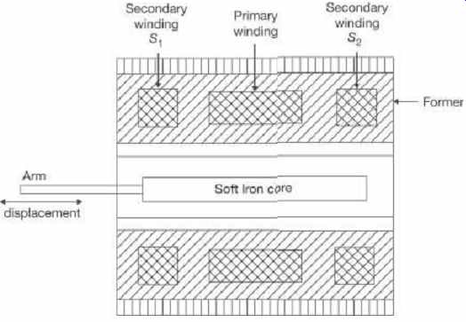
FIG. 1 Linear Variable Differential Transformer
(LVDT)
The primary winding is connected to an alternating current source. A movable soft-iron core is placed inside the former. The displacement to be measured is applied to the arm attached to the soft iron core. In practice the core is made of high permeability, nickel iron.
This is slotted longitudinally to reduce eddy current losses. The assembly is placed in a stainless steel housing to provide electrostatic and electromagnetic shielding. The frequency of ac signal applied to primary winding may be between 50 Hz to 20 kHz.
Since the primary winding is excited by an alternating current source, it produces an alternating magnetic field which in turn induces alternating voltages in the two secondary windings.
The output voltage of secondary S 1 is E S1 and that of secondary S 2 is E S2 . In order to convert the outputs from S 1 and S 2 into a single voltage signal, the two secondary S 1 and S 2 are connected in series opposition as shown in Figure 2. Differential output voltage
E 0 = E S1 − E S2
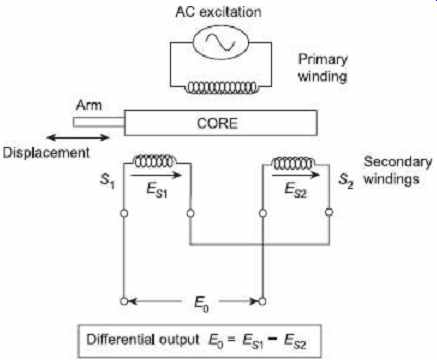
FIG. 2 Connection of LVDT circuit
3.1 Operation
When the core is at its normal (NULL) position, the flux linking with both the secondary windings is equal and hence equal emfs are induced in them. Thus, at null position: E S1 = E S2 . Thus, the output voltage E 0 is zero at null position.
Now if the core is moved to the left of the null position, more flux links with S 1 and less with winding S 2 . Accordingly, output voltages E S1 is greater than E S2 . The magnitude of output voltage is thus, E 0 = E S1 − E S2 and say it is in phase with primary voltage.
Similarly, when the core is moved to the right of the null position E S2 will be more than E S1 . Thus the output voltage is E 0 = E S1 − E S2 and 180° out of phase with primary voltage.
The amount of voltage change in either secondary winding is proportional to the amount of movement of the core. Hence, we have an indication of amount of linear motion. By noticing whether output voltage is increased or decreased, we can determine the direction of motion.
3.2 Advantages and Disadvantages of LVDT
Advantages
• Linearity is good up to 5 mm of displacement.
• Output is rather high. Therefore, immediate amplification is not necessary.
• Output voltage is stepless and hence the resolution is very good.
• Sensitivity is high (about 40 V/mm).
• It does not load the measurand mechanically.
• It consumes low power and low hysteresis loss also.
Disadvantages
• LVDT has large threshold.
• It is affected by stray electromagnetic fields. Hence proper shielding of the device is necessary.
• The ac inputs generate noise.
• Its sensitivity is lower at higher temperature.
• Being a first-order instrument, its dynamic response is not instantaneous.
Example 1 The output of an LVDT is connected to a 5 V voltmeter through an amplifier of amplification factor 250. The voltmeter scales has 100 divisions and the scale can be read to 1/5th of a division. An output of 2 mV appears across the terminals of the LVDT when the core is displaced through a distance of 0.5 mm. Calculate (a) the sensitivity of the LVDT, (b) that of the whole set up, and (c) the resolution of the instrument in mm.
Solution
(a) For a displacement of 0.5 mm, the output voltage is 2 mV.
Hence, the sensitivity of the LVDT is mV/mm = 4 mV/mm
(b) Due to the amplifier, this sensitivity is amplified 250 times in the set-up. Hence the sensitivity of the set-up is 4 × 250 = 1 V/mm
(c) The output of the voltmeter is 5 V with 100 divisions Each divisions corresponds to Since th of a division can be read, the minimum voltage that can be read is 0.01 V which corresponds to 0.01 mm. Hence, the resolution of the instrument is 0.01 mm.
4. STRAIN GAUGES
The strain gauge is an electrical transducer; it is used to measure mechanical surface tension. Strain gauge can detect and convert force or small mechanical displacement into electrical signals. On the application of force a metal conductor is stretched or compressed, its resistance changes owing to the fact both length and diameter of conductor change. Also, there is a change on the value of resistivity of the conductor when it is strained and this property of the metal is called piezoresistive effect. Therefore, resistance strain gauges are also known as piezoresistive gauges. The strain gauges are used for measurement of strain and associated stress in experimental stress analysis.
Secondly, many other detectors and transducers, for example the load cell, torque meter, flow meter, accelerometer employ strain gauge as a secondary transducer.
Theory of Resistance Strain Gauges
The change in the value of resistance by the application of force can be explained by the normal dimensional changes of elastic material. If a positive strain occurs, its longitudinal dimension ( x -direction) will increase while there will be a reduction in the lateral dimension ( y -direction). The reverse happens for a negative strain. Since the resistance of a conductor is directly proportional to its length and inversely proportional to its cross-sectional area, the resistance changes. The resistivity of a conductor is also changed when strained. This property is known as piezoresistive effect.
Let us consider a strain gauge made of circular wire. The wire has the dimensions:
length L , area A , diameter D before being strained. The material of the wire has a resistivity ρ .
Let a tensile stress S be applied to the wire. This produces a positive strain causing the length to increase and the area to decrease as shown in Figure 3 . Let Δ L = Change in length, Δ A = Change in area, Δ D = Change in diameter and Δ R is the change in resistance.
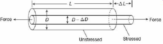
FIG. 3 Change in dimensions of a strain-gauge
element when subjected to a tensile force
In order to find how ΔR depends upon the material physical quantities, the expression for R is differentiated with respect to stress S . Thus, Dividing Eq. (1) throughout by resistance it becomes It is clear from Eq. (2) , that the per unit change in resistance is due to the following:
Per unit change in length =
Per unit change in area =
...and...
Per unit change in resistivity =
... or, putting this value of in Eq. (2) , it becomes
Now, Poisson's ratio
For small variations, the above relationship can be written as
The gauge factor is defined as the ratio of per unit change in resistance to per unit change in length.
where ε= = Strain
5. ELECTROMAGNETIC FLOW METER
Magnetic flow meters have been widely used in industry for many years. Unlike many other types of flow meters, they offer true non-invasive measurements. They are easy to install and use to the extent that existing pipes in a process can be turned into meters simply by adding external electrodes and suitable magnets. They can measure reverse flows and are insensitive to viscosity, density, and flow disturbances. Electromagnetic flow meters can rapidly respond to flow changes and they are linear devices for a wide range of measurements. In recent years, technological refinements have resulted in much more economical, accurate, and smaller instruments than the previous versions.
As in the case of many electric devices, the underlying principle of the electromagnetic flow meter is Faraday's law of electromagnetic induction. The induced voltages in an electromagnetic flow meter are linearly proportional to the mean velocity of liquids or to the volumetric flow rates. As is the case in many applications, if the pipe walls are made from nonconducting elements, then the induced voltage is independent of the properties of the fluid.
Figure 4 shows the schematic diagram of a Magnetic Meter (Magmeter), where V is the velocity of the liquid flow through the pipe, D is the internal diameter of the pipe, B is the flux density of the magnetic field and E s is the induced voltage at the electrodes due to the flow of the liquid through the pipe placed in the magnetic field.
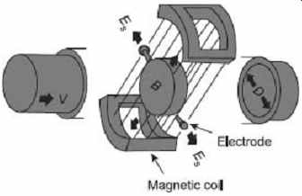
FIG. 4 The Magmeter and its components
The accuracy of these meters can be 0.25% at the best and, in most applications, an accuracy of 1% is used. At worst, 5% accuracy is obtained in some difficult applications where impurities of liquids and the contact resistances of the electrodes are inferior as in the case of low-purity sodium liquid solutions.
5.1 Faraday's Law of Induction
This law states that if a conductor of length l (m) is moving with a velocity v (m/s), perpendicular to a magnetic field of flux density B (Tesla) then the induced voltage across the ends of conductor can be expressed by
The principle of application of Faraday's law to an electromagnetic flow meter is given in Figure 5. The magnetic field, the direction of the movement of the conductor, and the induced emf are all perpendicular to each other.
Figure 6 illustrates a simplified electromagnetic flow meter in greater detail.
Externally located electromagnets create a homogeneous magnetic field (B) passing through the pipe and the liquid inside it. When a conducting flowing liquid cuts through the magnetic field, a voltage is generated along the liquid path between two electrodes positioned on the opposite sides of the pipe.
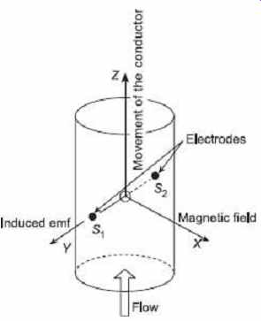
FIG. 5 Operational principle of electromagnetic
flow meters
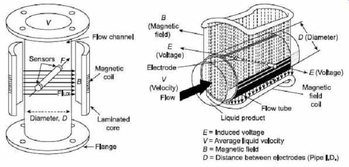
FIG. 6 Construction of practical flow meters
In the case of electromagnetic flow meters, the conductor is the liquid flowing through the pipe, and the length of the conductor is the distance between the two electrodes, which is equal to the tube diameter (D). The velocity of the conductor is proportional to the mean flow velocity (v) of the liquid. Hence, the induced voltage becomes ...
If the magnetic field is constant and the diameter of the pipe is fixed, the magnitude of the induced voltage will only be proportional to the velocity of the liquid. If the ends of the conductor, in this case the sensors, are connected to an external circuit, the induced voltage causes a current, i to flow, which can be processed suitably as a measure of the flow rate. The resistance of the moving conductor can be represented by R to give the terminal voltage as v T = e − iR.
Electromagnetic flow meters are often calibrated to determine the volumetric flow of the liquid. The volume of liquid flow, Q can be related to the average fluid velocity as ...
Writing the area, A of the pipe as gives the induced voltage as a function of the flow rate.
Equation (11) indicates that in a carefully designed flow meter, if all other parameters are kept constant, then the induced voltage is linearly proportional to the liquid flow only.
Based on Faraday's law of induction, there are many different types of electromagnetic flow meters available, such as ac, dc, and permanent magnets. The two most commonly used ones are the ac and dc types. This section concentrates mainly on ac and dc type flow meters.
Although the induced voltage is directly proportional to the mean value of the liquid flow, the main difficulty in the use of electromagnetic flow meters is that the amplitude of the induced voltage is small relative to extraneous voltages and noise.
Noise sources include:
• Stray voltage in the process liquid
• Capacitive coupling between signal and power circuits
• Capacitive coupling in connection leads
• Electromechanical emf induced in the electrodes and the process fluid
• Inductive coupling of the magnets within the flow meter
Advantages of Electromagnetic Flow Meter
• The electromagnetic flow meter can measure flow in pipes of any size provided a powerful magnetic field can be produced.
• The output (voltage) is linearly proportional to the input (flow).
• The major advantage of electromagnetic flow meter is that there is no obstacle to the flow path which may reduce the pressure.
• The output is not affected by changes in characteristics of liquid such as viscosity, pressure and temperature.
Limitations
• The operating cost is very high in an electromagnetic flow meter, particularly if heavy slurries (solid particle in water) are handled.
• The conductivity of the liquid being metered should not be less than 10 μΩ/m. It will be found that most aqueous solutions are adequately conductive while a majority of hydrocarbon solutions are not sufficiently conductive.
5.2 Comparison of dc and ac Excitation of Electromagnetic Flow Meter
The magnetic field used in electromagnetic flow meter can either be ac or dc giving rise to ac or a dc output signal respectively. The dc excitation is used in few applications due to the following limitations of the dc excitation.
When dc excitation is used for materials of very low conductivity and flowing at slow speeds, the output emf is too small to be easily read off. The dc amplifiers used in this purposes are also have some inherent problems especially at low level.
Many hydrocarbon or aqueous solutions exhibit polarization effects when the excitation is dc. The positive ions migrate to the negative electrode and disassociate, forming an insulating pocket of gaseous hydrogen, there is no such phenomena when ac is used.
The dc field may distort the fluid velocity profile by Magneto Hydro Dynamic (MHD) action. An ac field of normal frequency (50 Hz) has little effect on velocity profile because fluid inertia and friction forces at 50 Hz and sufficient to prevent any large fluid motion.
Since the output of electromagnetic flow meters is quite small (a few mV), interfering voltage inputs due to thermocouple type of effects and galvanic action of dissimilar metals used in meter construction may be of the same order as the signal. Since the spurious interfering inputs are generally drifts of very low frequency, the 50 Hz system can use high pass filters to eliminate them.
While ac system predominates, dc types of systems have been used for flow measurements of liquid metals like mercury. Here, no polarization problem exists. Also, an insulating pipe or a nonmetallic pipe is not needed since the conductivity of the liquid metal is very good relative to an ordinary metal pipe. This means that the metal pipe is not very effective as a short circuit for the voltage induced in the flowing liquid metal. When metallic pipes are used as with dc excitation no special electrodes are necessary. The output voltage is tapped off the metal pipe itself at the points of maximum potential difference.