AMAZON multi-meters discounts AMAZON oscilloscope discounts
<< cont. from part 4
5.8 Thermometer Lag
Liquid-in-glass thermometers require a finite amount of time to achieve a final, equilibrium temperature. The time required can vary for individual thermometer types depending on the diameter of the thermometer, the size and volume of the bulb, the heat conductivity of the material into which the thermometer is placed, and the circulation rate of that material.
For taking the temperature of a material that maintains a constant-temperature, thermometer lag is only a nuisance. Most laboratory thermometers placed in a 75°C bath will come within 0.01°C of the final temperature within 19 to 35 seconds of first contact. The time range is dependent on the type and design of the thermometer.
When attempting to measure a changing temperature, the problem is more critical because you are limited to knowing what the temperature was, not is. Because of the thermometer's lag time, you will be unable to know any specific tempera ture instantaneously. Thus, the greater the rate of temperature increase, the less a thermometer is able to keep up with the temperature change. Interestingly enough, if the temperature change varies uniformly, White found that any thermometer lag is likely to be canceled because any rate of change will not have been altered.
5.9 Air Bubbles in Liquid Columns
Sometimes, because of shipping, general use, or sloppy handling, the liquid column of a thermometer will separate, leaving trapped air bubbles. Because of the capillary size, it is difficult for the liquid to pass by the air space and rejoin. Some times such separations are glaringly obvious. Other times, the amount of liquid separation is small and is difficult to see.
One technique for monitoring the quality of a thermometer is to use a second thermometer for all measurements. Any disagreement between the temperatures from the two thermometers may be caused by a problem as air breaks in the liquid columns. If both thermometers have breaks in their liquid columns, it is almost impossible for them to agree across a range of temperatures. Detection of liquid breaks is virtually guaranteed. Unfortunately, this technique will not identify which thermometer is at fault.
There are two techniques for rejoining separated liquid ends: heating and cooling. The option chosen will depend on the location of the break, as well as on the existence and location of contraction or expansion chambers.
Generally it is better (and safer) to cool the liquid in thermometer than it is to heat it. First, try to cool the thermometer with a (table) salt-and-ice slush bath.* This method should bring the liquid into the contraction chamber or bulb. Once the liquid is in the chamber or bulb, it should rejoin, leaving the air bubble on top.
If there is not a clean separation of the air bubble, it may be necessary to softly tap the end of the thermometer. This tapping should be done on a soft surface such as a rubber mat, stopper, or even a pad of paper. Alternatively, you may try swinging the thermometer in an arc (such as a nurse does before placing it in your mouth)." Once joined, the liquid in the thermometer can slowly be reheated.
If the scale or design of the thermometer is such that these methods will not work, try touching the bulb end to some dry ice. Because dry ice is 38°C colder than the freezing point of mercury, you must pay attention and try to prevent the mercury from freezing. As a precaution, when reheating, warm from the top (of the bulb) down to help prevent a solid mercury ice plug from blocking the path of the expanding mercury into the capillary. With no path to expand into, the expanding liquid may otherwise cause the bulb to explode.
An alternate technique to rejoin broken liquid columns is to expand the liquid into the contraction or expansion chamber by heat. Be careful to avoid filling the expansion chamber more than two-thirds full, as extra pressure may cause the top of the thermometer to burst. Never use an open flame to intentionally heat any part of a thermometer as the temperature from such a source is too great and generally uncontrollable.
[This assumes that the location of 0°C is sufficiently close to either the bulb or the contraction chamber; otherwise a different slush bath may be required.
Medical thermometers have a small constriction just above the bulb that serves as a gate valve. The force of the mercury expanding is great enough to force the mercury past the constriction. However, the force of contraction is not great enough to draw the mercury back into the bulb. The centrifugal force caused by shaking the thermometer is great enough to draw the mercury back into the bulb.]
If the thermometer has no expansion or contraction chamber, heating the bulb should not be attempted because there is no place into which the liquid may expand to remove bubbles. Occasionally it may be possible to heat the upper region of the liquid along the stem (do not use a direct flame; use a hot air gun or steam). Observe carefully, and look for the separated portion to break into small balls on the walls of the capillary. These balls may be rejoined to the rest of the liquid by slowly warming the bulb of the thermometer so that the microdroplets are gathered by the expanding mercury. Once collected, the mercury may be slowly cooled.
In addition to air bubbles in the stem, close examination of the thermometer bulb may reveal small air bubbles in the mercury. Carefully cool the mercury in the bulb until the liquid is below the capillary. While holding the thermometer horizontal, tap the end of the thermometer against your hand (you are trying to form a bubble within the bulb). Next, rotate the thermometer, allowing the large air bubble to contact the internal surface of the bulb, capturing the small air bubbles. Once the small air bubbles are "caught," the thermometer can be reheated as before.
IMPORTANT: Many states are limiting the use of mercury in the laboratory.
Such laws severely limit the use of mercury-in-glass thermometers despite the fact that the mercury is isolated from the environment in normal use. Unfortunately, the laws apply because a broken thermometer can easily release its mercury into the lab. Fortunately, thermocouples (see Sec. 2.5.11) are relatively inexpensive, and the price of controllers has gone down significantly-while the accuracy of thermocouples and the ease of their use have gone up significantly. Thermocouples should be considered as an alternative even if you are not receiving pressure to reduce mercury use because of ease of use and robust design.
5.10 Pressure Expansion Thermometers
Gas law theory maintains that pressure, volume, and temperature have an interdependent relationship. If one of these factors is held constant and one changes, the third has to change to maintain an equilibrium. At low temperatures and pressures, gases follow the standard gas law equation much better than they do at other conditions [see Eq. (eqn. 7)].
PV=nRT (eqn. 7)
where P = pressure (in torr) and V = Volume (in liters)
n = number of molecules
R = gas constant (62.4)
T = temperature (in K)
The typical pressure expansion thermometer is a volume of gas that maintains the same number of molecules throughout a test. Because the volume, number of molecules, and gas constant are all constant, any drop in temperature will subsequently cause a drop in pressure. Likewise, any rise in temperature will cause a rise in pressure.
These thermometers are difficult to use, are sensitive, and require a great deal of supporting equipment. They are typically used for the calibration of other (easier to use) thermometers. In addition, they are used to determine the temperatures of melting, boiling, and transformation points of various materials. Because of their limited use in the average laboratory, further discussion of pressure expansion thermometers is beyond the scope of this guide.
5.11 Thermocouples
Thermocouples are robust and inexpensive. Reading the temperature from a thermocouple is invariably as easy as reading a controller's dial, liquid crystal, or LED. The following commentary is intended to provide a basic understanding of the operation of thermocouples and their limitations. If you have any questions about the final selection of a thermocouple, controller, lead, and extension for any specific type of job or desired use, contact a thermocouple manufacturing company because it will likely provide you with the best information on how to make your system work.

Table 33 Thermocouple Types and Characteristics
[LED stands for light emitting diode. These devices are the lighted numerals typically seen on digital clocks.]
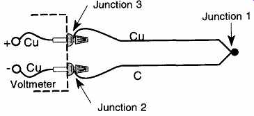
FIG. 31 A simple diagram of a copper-constantan thermocouple. This illustration
is from The Temperature Handbook©1989 by Omega Engineering, Inc.
In 1821 Thomas Seebeck discovered that when two different types of metal wires were joined at both ends and one of the ends was heated or cooled, a current was created within the closed loop (this current is now called the Seebeck effect). Specifically, heat energy was transformed into measurable electrical energy.
Unfortunately, there is not enough current produced to do any work, but there is enough to measure (1 to 7 millivolts). This rise in potential energy is called the emf or electromotive force.
By hooking the other end of joined dissimilar wires up to a voltmeter and measuring the emf (output), it is possible to determine temperature. Such a tempera ture-measuring device is called a thermocouple.
There are seven common thermocouple types as identified by the American National Standards Institute (ANSI). They are identified by letter designation and are described in Table 33. There are four other thermocouple types that have letter designations; however, these four are not official ANSI code designations because one or both of their paired leads are proprietary alloys. They are included at the end of Table 33. Although Table 33 lists the standard commercially available thermocouples, there are technically countless other potential thermocouples because all that is required for a thermocouple is two dissimilar wires.
At a basic level, it seems that one should be able to take any thermocouple, attach it to a voltmeter, and determine the amount of electricity generated from the heat applied to the dissimilar junction. Then the user could look in some predetermined thermocouple calibration table to determine the amount of heat that the amount of electricity from that specific type of joined wires produces.
[Thermocouple calibration tables have been compiled by the NIST and can be found in a variety of sources such as the Handbook of Chemistry and Physics by the Chemical Rubber Company, published yearly.]
One of the negative complications of thermocouples is that they do not have a linear response to heat. In addition, as temperature changes, thermocouples do not produce a consistent emf change. Therefore, there must be individual thermocouple calibration tables for each type of thermocouple.
If you look at a thermocouple calibration table, you will see that it has a reference junction at 0°C. This reference point is used because of an interesting complication that arises when a thermocouple is hooked up to a voltmeter. To explain this phenomenon, first look at one specific type of thermocouple, a type T (copper-constantan design). Also, assume that the wires in the voltmeter are all copper.
Once the thermocouple is hooked to the voltmeter, we end up having a total of three junctions (see FIG. 31):
Junction 1. The original thermocouple junction of copper and constantan.
Junction 2. The connection of the constantan thermocouple wire to the copper wire of the volt meter.
Junction 3. The connection of the copper thermocouple wire to the copper wire of the volt meter.
We are hoping to find the temperature of Junction 1, but it seems we now have two more junctions with which to be concerned. Fortunately, Junction 3 can be ignored because this connection is of similar, not dissimilar, metals. Therefore, no emf will be produced at this junction. Junction 2 presents a problem because it will produce an emf, but of an unknown temperature; this means that we have two unknowns in the same circuit, and we are unable to differentiate between the two.
Any voltmeter reading taken at this point will be proportional to the temperature difference between the first and third junction.
If we take Junction 2 and place it in a known temperature, we can eliminate one of the two unknowns. This procedure is done by placing Junction 2 (now known as the reference junction) in an ice bath of 0°C (known as the reference tempera ture). Because the temperature (voltmeter) reading is based on an ice-bath reference temperature, the recording temperature is referenced to 0°C (see FIG. 32).
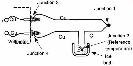
FIG. 32 A thermocouple using an ice bath for a reference temperature.
References for voltmeter/thermocouple readings (found in such books as the CRC Handbook) will usually indicate that they are referenced to 0°C. Because Junctions 3 and 4 are of similar metals, they have no effect on the emf.
This example is limited because it is representative only of thermocouples with copper leads. In all other thermocouples, there are likely to be four dissimilar metal junctions and therefore up to four Seebeck effects. However, by extending the copper wires from the voltmeter and attaching them to an isothermal block, placing the same type of wire from one of the thermocouple leads to the part between the ice-bath and the isothermal block, and then attaching the thermocouple wires to the isothermal block (to eliminate thermal differences at these two junctions), it is possible to cancel out all but the desired Seebeck effect (see FIG. 33).
It is obvious that the use of an ice bath is inconvenient and impractical. Maintaining a constant 0.0°C temperature can be difficult, and there always is the possibility of the icebath tipping over. Fortunately there are two convenient techniques to circumvent the need for an actual ice bath for thermocouple measurements.
One approach requires measuring the equivalent voltage of the ice-bath reference junction and having a computer compensate for the equivalent effect. This technique, called software compensation, is the most robust and easiest to use.
However, depending on the equipment used, the lag time involved for the compensation may be unacceptable.
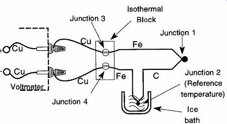
FIG. 33 An iron-constantan thermocouple using an isothermal block and
an ice bath.
Alternatively, it is possible to have hardware compensation by inserting an electric current (typically from a battery) to provide a voltage which electronically offsets the reference junction. This approach is called an electronic ice-point reference. This method has the simplicity of an ice bath, but is far more convenient to use. The major disadvantage is that a different electric circuit is required for each type of thermocouple.
Ironically, the sophistication of modern controllers typically makes most of the concerns about how temperature is determined irrelevant. The greatest concern for the user is to select the right type and size of thermocouple for the specific job and environment, then to select the proper controller for that type of thermocouple.
Although there are many overlapping temperature ranges among various thermocouple types, all types of thermocouples perform better for some jobs than others. For example, Type K is significantly less expensive than Type R, although both thermocouples can read into the 1000°C range. This similarity would lead one to believe that either choice is adequate, however Type K is preferred because of its lower cost. If all you need are occasional readings of such temperatures, you could get by with Type K. However, if you expect to do repeated and constant cycling up to temperatures in the 1000°C range, Type K would soon fail and would need to be replaced. Unfortunately, you are not likely to notice failure developing until something has obviously gone wrong. Because the potential costs of failure are likely to be greater than the additional cost of the more expensive thermocouple, it may be more economical to obtain the more expensive type R at the outset.
Sample size should also be considered when selecting thermocouple size. If a large thermocouple (with a high heat capacitance) is used on a small sample (with a low heat capacitance), the sample's temperature could be changed. As stated before, the act of taking an object's temperature can change its temperature.
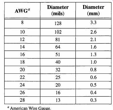
Table 34 American Wire Gauge Size Comparison Chart
American Wire Gauge.
Because thermocouples come with varying wire diameters (see Table 34), select the thermocouple wire size best suited to measure your sample.
Be advised that the upper range of temperatures cited (within thermocouple catalogs) for a given thermocouple are related to the larger wire sizes. Thus, a small wire thermocouple is likely to fail at the upper temperature ranges for that particular thermocouple type.
Environment also influences the selection of thermocouples. The condition of the region where the thermocouple will be placed can be oxidizing, reducing, moist, acidic, or alkaline, or it can present some other condition that could cause premature failure of the thermocouple. Selection of the right type of thermocouple can help avoid premature failure. Fortunately, there are sleeves and covers avail able for thermocouples that prevent direct contact with their various environments. These covers are made of a variety of materials, from metals to ceramics, making selection of the right material easy. On the other hand, covers add to the heat capacitance of the entire probe and therefore can slow thermocouple response time; and because of a greater heat capacity, they are more likely to affect the temperature of the material being studied.
5.12 Resistance Thermometers
In 1821, Sir Humphrey Davy discovered that as temperature changed, the resistance of metals changed as well. By 1887 H.L. Callendar completed studies showing that purified platinum wires exhibited sufficient stability and reproducibility for use as thermometer standards. Further studies brought the Comite International des Poids et Measures in 1927 to accept the Standard Platinum Resistance Thermometer (SPRT) as a calibration tool for the newly adopted practical temperature scale.
Platinum resistance thermometers are currently used by the NIST for calibration verification of other thermometer types for the temperature range 13.8 to 904 K.
In addition, they are one of the easiest types of thermometers to interface with a computer for data input. On the other hand, platinum resistance thermometers are very expensive, extremely sensitive to physical changes and shock, have a slow response time, and therefore can take a long time to equilibrate to a given temperature. Thus, resistance thermometers are often used only for calibration purposes in many labs.
Platinum turned out to be an excellent choice of materials because it can with stand high heat and is very resistant to corrosion. In addition, platinum offers a reasonable amount of resistivity (as opposed to gold or silver), yet it is very stable and its resistance is less likely to drift with time. However, because it is a good conductor of electricity, the SPRT requires a sufficiently long enough piece of platinum wire* to record any resistance.
One of the easiest ways to get a long piece of material in a small (convenient) area is to wrap or wind the material around a mandrel. The typical mandrel used on SPRTs is made of either mica or alumina. The sheaths covering the wrapped thermometer may be borosilicate, silica glass, or a ceramic (see FIG. 33). Note that both examples in FIG. 33 show four leads where, logically, there should be only two. This is done to reduce any unwanted resistance from the region beyond the thermometer.
[Currently, about 61 cm of 0.075-mm platinum wire is typically used on resistance thermometers.]
An alternative approach to "loose winding" the wires is to form the platinum wire and then flow melted glass around the wire to "lock" the wire in place. This method protects the wire from shock and vibration. These resistance thermometers are, unfortunately, limited to temperatures where the expanding platinum will not crack the containment glass. To limit this occurrence, the expansion of the platinum must closely match the glass around which it is wrapped. Resistance thermometers of this design are more rugged, and therefore, they are more likely to be used in the laboratory.
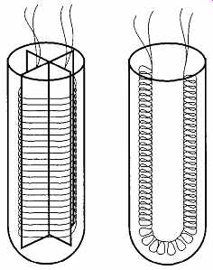
FIG. 34 Two different SPRT wrapping designs.
There are many challenges in the construction and use of resistance thermometers, including:
1. The wire itself must be very pure; any impurities will affect the linearity and reliability of the resistance change. The wire itself must also be uniformly stressed, meaning that after construction, the wire must be temperature-annealed to achieve uniform density. Uniform density provides uniform resistance.
2. When the wire is wound on the support device, it must be left in a strain free condition, as any strain can also affect the resistance of metals.
Because the platinum will expand and contract as the temperature changes, it must be wound in such a manner that there is no hold-up or strain. Even this strain could affect the resistance of the metal.
3. Although it is doubtful that a lab will make its own SPRTs, I mention construction demands to impress upon the user the importance of maintaining a strain-free platinum wire. Strain on the wire can be introduced not only during construction, but also in use. The most likely opportunities for wire strain are through vibration and bumping.
4. The SPRT must not receive any sharp motions or vibrations. Such actions can affect the resistance of the metal by creating strain. To place this challenge in the proper perspective, consider a SPRT rapped against a solid surface loud enough to be heard (but not hard enough to fracture the glass sheath). The temperature readings could be affected by as much as 0.001 °C. Although this variation may not seem like much, over a year's time, such poor use could cause as much as 0.1 °C error.
Transportation of SPRTs should be as limited as possible. If you are shipping, special shock-absorbing boxes are recommended. If you have an SPRT shipped to you, keep the box for any future shipping needs and storage. Calibrated SPRTs should be hand-carried whenever possible, to minimize shock or vibration. For instance, you should not lay an SPRT on a lab cart for transportation down the hall. The vibration of the cart may cause changes in subsequent temperature readings.
Other precautions that should be taken with SPRTs include the following:
1. When SPRTs are placed into an apparatus, they should be inserted care fully, to avoid bumps and shocks.
2. Try to avoid rapid dramatic changes in temperature. A cold-to-hot change can cause strains as the wire expands within the thermometer.
A hot-to-cold change can cause fracture of the glass envelope encasing the thermometer, or of any glass-to-metal seals (which are structurally weak). A hot-to-cold heat change can also cause a calibration shift of the thermometer.
3. Thermometers with covers of borosilicate glass should not be used in temperatures over 450-500°C without some internal support to pre vent deformation.
4. Notable grain growth has been observed in thermometers maintained at 420°C for several hundred hours.
Such grain growth causes the thermometer to be more susceptible to calibration changes from physical shock and therefore, inherently unstable.
There are several inherent complications in the use of SPRTs. One involves the fact that an SPRT is not a passive responding device. What the SPRT records is the change in resistance of an electric current going through the thermometer. The mere fact that you are creating resistance means that you are creating heat. Thus, the device that is designed to measure heat also creates heat. The resolution of this situation is to 1) use as low a current as possible to create as little heat as possible and 2) use as large an SPRT as possible (the larger the SPRT, the less heat generated).
Although an SPRT is not a thermocouple, an emf is created at the junction of the SPRT's platinum wires and the controller's copper wires. Fortunately, this emf is automatically dealt with electronically by the controller with the offset-compensation ohms technique and can be ignored by the user.
References
1. Verney Stott, Volumetric Glassware H.F. & G. Witherby, London, 1928, pp. 13-14.
2. R.B. Lindsay, "The Temperature Concept for Systems in Equilibrium" in Tempera ture; Its Measurement and Control in Science and Industry, Vol. 3, F.G. Brick wedde, ed., Part 1, Reinhold Publishing Corporation, New York, 1962, pp. 5-6.
3. W.E. Knowles Middleton, A History of the Thermometer and Its Use in Meteorology, The John Hopkins Press, Baltimore, Maryland, 1966, pp. 58-61.
4. A.V. Astin, "Standards of Measurement," Scientific American, 218, pp. 50-62 (1968).
5. E. Ehrlich, et al, Oxford American Dictionary Oxford University Press, 1980.
6. D.R. Burfield and G. Hefter, "Oven Drying of Volumetric Glassware," Journal of Chemical Education, 64, p. 1054 (1987).
7. H.P. Williams and F.B. Graves, "A Novel Drying/Storage Rack for Volumetric Glassware," J. of Chem. Ed., 66, p. 771 (1989).
8. D.J. Austin, "Simple Removal of Buret Bubbles," Journal of Chemical Education, 66, p. 514(1989).
9. Dr. L. Bietry, Mettler, Dictionary of Weighing Terms, Mettler Instrumente AG, Switzerland, 1983, p. 12.
10. W.E. Kupper, "Validation of High Accuracy Weighing Equipment," Proceedings of Measurement Science Conference 1991, Anaheim, CA.
11. R.M. Schoonover and F.E. Jones, "Air Buoyancy Correction in High-Accuracy Weighing on Analytical Balance," Analytic Chemistry, 53, pp. 900-902 (1981).
12. W.E. Kupper, "Honest Weight - Limits of Accuracy and Practicality," Proceedings of Measurement Science Conference 1990, Anaheim, CA.
13. From "Weighing the Right Way with METTLER," © 1989 by Mettler Instrumente AG, printed in Switzerland.
14. Ibid, Ref. 9, pp. 69. 74, 100, and 118.
15. Jacquelyn A. Wise, Liquid-in-Glass Thermometry, U.S. Government Printing Office, Washington, D.C., 1976, p. 23.
16. E.L. Ruh and G.E. Conklin, "Thermal Stability in ASTM Thermometers," ASTM Bulletin, No. 233, p. 35, Oct. 1958.
17. W.I. Martin and S.S. Grossman, "Calibration Drift with Thermometers Repeatedly Cooled to -30° C," ASTM Bulletin, No. 231, p. 62, July, 1958.
18. W.P. White, "Lag Effects and Other Errors in Calorimetry," Physical Review, 31, pp. 562-582 (1910).
19. J.L. Riddle, G.T. Furukawa, and H.H. Plumb, Platinum Resistance Thermometry, National Bureau of Standards Monograph No. 126, U.S. Government Printing Office, April 1972, p. 9.
20. Ibid, Ref. 19, p. 11.