AMAZON multi-meters discounts AMAZON oscilloscope discounts
This section explores a device that has applications in general RF electronics as well as in antenna work: the RF noise bridge. It is one of the most useful, low-cost, and over-looked test instruments in the servicer's armamentarium.
Several companies have produced low-cost noise bridges: Omega-T, Palomar Engineers, and the now out-of-the-kit-business Heath Company. The Omega-T device (Fig. 17-1A) is a small cube with minimal dials and a pair of BNC coax connectors (marked antenna and receiver). The dial is calibrated in ohms and measures only the resistive component of impedance. The Palomar Engineers device (Fig. 17-1B) is a little less eye-appealing but does everything the Omega-T does, plus it allows you to make a rough measurement of the reactive component of impedance.
The Heath Company had their Model HD-1422 in the line-up. Over the years, I have found the noise bridge terribly useful for a variety of test and measurement applications-especially in the HF and low-VHF regions, and those applications are not limited to the testing of antennas (which is the main job of the noise bridge). In fact, the two-way technician (including CB) will measure antennas with the device, but consumer technicians will find other applications.
Figure 17-2 shows the block diagram of this instrument. The bridge consists of four arms. The inductive arms (L1b and L1c) form a trifilar-wound transformer over a ferrite core with L1a so signals applied to L1a are injected into the bridge circuit. The measurement consists of a series circuit with a 200-ohm potentiometer and a 120-pF variable capacitor. The potentiometer sets the range (0 to 200 ohm) of the resistive component of measured impedance and the capacitor sets the reactance component. Capacitor C2 in the UNKNOWN arm of the bridge is used to balance the measurement capacitor. With C2 in the circuit, the bridge is balanced when C is approximately in the center of its range. This arrangement accommodates both inductive and capacitive reactances, which appear on either side of the "zero" point (i.e., the mid-range capacitance of C). When the bridge is in balance, the settings of R and C reveal the impedance across the UNKNOWN terminal.
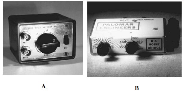
17-1 (A) Omega-T noise bridge and (B) Palomar noise bridge.
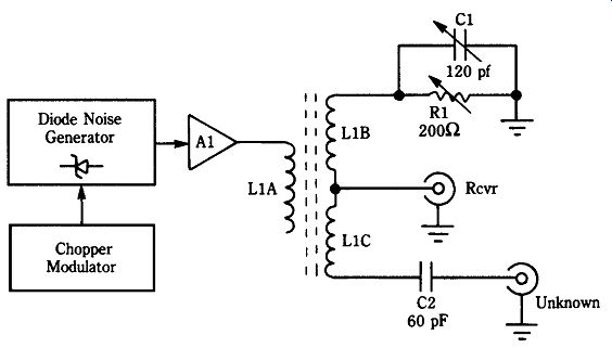
17-2 Block diagram of an RF noise bridge.
A reverse-biased zener diode (zeners normally operate in the reverse bias mode) produces a large amount of noise because of the avalanche process inherent in zener operation. Although this noise is a problem in many applications, in a noise bridge it is highly desirable: the richer the noise spectrum the better. The spectrum is enhanced somewhat in some models because of a 1-kHz square-wave modulator that chops the noise signal. An amplifier boosts the noise signal to the level needed in the bridge circuit.
The detector used in the noise bridge is a HF receiver. The preferable receiver uses an AM demodulator, but both CW (Morse code) and SSB receivers will do in a pinch. The quality of the receiver depends entirely on the precision with which you need to know the operating frequency of the device under test.
Adjusting antennas
Perhaps the most common use for the antenna noise bridge is finding the impedance and resonant points of a HF antenna. Connect the RECEIVER terminal of the bridge to the ANTENNA input of the HF receiver through a short length of coaxial cable as shown in Fig. 17-3. The length should be as short as possible, and the characteristic impedance should match that of the antenna feedline. Next, connect the coaxial feedline from the antenna to the ANTENNA terminals on the bridge. You are now ready to test the antenna.
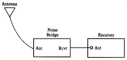
17-3 Connection of the noise bridge to the receiver and antenna
Finding impedance
Set the noise bridge resistance control to the antenna feedline impedance (usually 50 or 75 ohm for most amateur antennas). Set the reactance control to mid-range (zero). Next, tune the receiver to the expected resonant frequency (Fexp) of the antenna. Turn the noise bridge on and look for a noise signal of about S9 (will vary on different receivers and if in the unlikely event that the antenna is resonant on the expected frequency).
Adjust the resistance control (R) on the bridge for a null (i.e., minimum noise, as indicated by the S meter). Next, adjust the reactance control (C) for a null. Re peat the adjustments of the R and C controls for the deepest possible null, as indicated by the lowest noise output on the S meter (there is some interaction between the two controls).
A perfectly resonant antenna will have a reactance reading of zero _ and a resistance of 50 to 75 ohm . Real antennas might have some reactance (the less the better) and a resistance that is different from 50 or 75 ohm . Impedance-matching methods can be used to transform the actual resistive component to the 50- or 75-ohm characteristic impedance of the transmission line.
If the resistance is close to zero, suspect that there is a short circuit on the trans mission line and an open circuit if the resistance is close to 200 ohm.
A reactance reading on the XL side of zero indicates that the antenna is too long and a reading on the Xc side of zero indicates an antenna that is too short.
An antenna that is too long or too short should be adjusted to the correct length.
To determine the correct length, we must find the actual resonant frequency, Fr. To do this, reset the reactance control to zero and then slowly tune the receiver in the proper direction-downband for too long and upband for too short-until the null is found. On a high-Q antenna, the null is easy to miss if you tune too fast. Don't be surprised if that null is out of band by quite a bit. The percentage of change is given by dividing the expected resonant frequency (Fexp) by the actual resonant frequency (Fr) and multiplying by 100:

(17-1)
Resonant frequency
Connect the antenna, noise bridge, and the receiver in the same manner as above. Set the receiver to the expected resonant frequency (i.e., 468/F for half wavelength types and 234/F for quarter-wavelength types). Set the resistance control to 50 or 75 ohm , as appropriate for the normal antenna impedance and the transmission-line impedance. Set the reactance control to zero. Turn the bridge on and listen for the noise signal.
Slowly rock the reactance control back and forth to find on which side of zero the null appears. Once the direction of the null is determined, set the reactance control to zero then tune the receiver toward the null direction (downband if null is on the XL side and upband if on the Xc side of zero).
A less-than-ideal antenna will not have exactly 50 or 75 ohm of impedance so you must adjust R and C to find the deepest null. You will be surprised how far off some dipoles and other forms of antennas can be if they are not in "free space" (i.e., if they are close to the Earth's surface).
Non-resonant antenna adjustment
We can operate antennas on frequencies other than their resonant frequency if we know the impedance. For the antenna to radiate properly, however, it is necessary to match the impedance of the antenna feedpoint to the source (e.g., a trans mission line from a transmitter). We can find the feedpoint resistance from setting the potentiometer in the noise bridge. The reactances can be calculated from the reactance measurement on the bridge by looking at the capacitor setting-and using a little arithmetic:
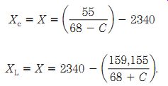
(17-2)
Now, plug "X" calculated from one of the previous equations into Xf _ X/F, where F is the desired frequency in megahertz.
Other RF jobs for the noise bridge
The noise bridge can be used for a variety of jobs. We can find the values of capacitors and inductors, the characteristics of series and parallel-tuned resonant circuits, and the adjustment transmission lines.
Transmission line length
Some antennas and (non-noise) measurements require antenna feedlines that are either a quarter-wavelength or a half-wavelength at some specific frequency. In other cases, a piece of coaxial cable of specified length is required for other purposes: for instance, the dummy load used to service-depth sounders is nothing, but a long piece of shorted coax that returns the echo at a time interval that corresponds to a specific depth. We can use the bridge to find these lengths as follows:
1. Connect a short-circuit across the UNKNOWN and adjust R and X for the best null at the frequency of interest (note: both will be near zero).
2. Remove the short-circuit.
3. Connect the length of transmission line to the unknown terminal-it should be longer than the expected length.
4. For quarter-wavelength lines, shorten the line until the null is very close to the desired frequency. For half-wavelength lines, do the same thing, except the line must be shorted at the far end for each trial length.
Transmission-line velocity factor
The velocity factor of a transmission line (usually designated by V in equations) is a decimal fraction that tells us how fast the radiowave propagates along the line relative to the speed of light in free space. For example, foam dielectric coaxial cable is said to have a velocity factor of V = 0.80. This number means that the signals in the line travel at a speed 0.80 (or 80%) of the speed of light.
Because all radio-wavelength formulas are based on the velocity of light, you need the V value to calculate the physical length needed to equal any given electrical length. For example, a half wavelength piece of coax has a physical length of
[(492)(V)/FMHz] ft.
Unfortunately, the real value of V is often a bit different from the published value. You can use the noise bridge to find the actual value of V for any sample of coaxial cable:
1. Select a convenient length of the coax (more than 12 ft in length) and install a PL-259 RF connector (or other connector compatible with your instrument) on one end and short-circuit the other end.
2. Accurately measure the physical length of the coax in feet; convert the "remainder" inches to a decimal fraction of 1 ft by dividing by 12 (e.g., 32_ 8__ 32.67_ because 8_/12__ 0.67). Alternatively, cut off the cable to the nearest foot and reconnect the short circuit.
3. Set the resistance and reactance controls to zero.
4. Adjust the monitor receiver for deepest null. Use the null frequency to find the velocity factor, V _ FL/492, where V is the velocity factor (a decimal fraction), F is the frequency in megahertz, and L is the cable length in feet.
Tuned circuit measurements
An inductor/capacitor (LC) tuned "tank" circuit is the circuit equivalent of a resonant antenna so there is some similarity between the two measurements. You can measure resonant frequency with the noise bridge to within _20% or better if care is taken. This accuracy might seem poor, but it is better than one can usually get with low-cost signal generators, dip meters, absorption wave meters, and so on.
Series-tuned circuits
A series-tuned circuit exhibits a low impedance at the resonant frequency and a high impedance at all other frequencies. Start the measurement by connecting the series-tuned circuit under test across the unknown terminals of the bridge. Set the resistance control to a low resistance value, close to 0 _. Set the reactance control at mid-scale (zero mark). Next, tune the receiver to the expected null frequency then tune for the null. Be sure that the null is at its deepest point by rocking the R and X controls for best null. At this point, the receiver frequency is the resonant frequency of the tank circuit.
Parallel resonant-tuned circuits
A parallel resonant circuit exhibits a high impedance at resonance and a low impedance at all other frequencies. The measurement is made in exactly the same manner, as for the series resonant circuits, except that the connection is different.
Figure 17-4 two-turn link coupling is needed to inject the noise signal into the parallel resonant tank circuit. If the inductor is the toroidal type then the link must go through the hole in the doughnut-shaped core and then connect to the UNKNOWN terminals on the bridge. After this, do exactly as you would for the series-tuned tank measurement.
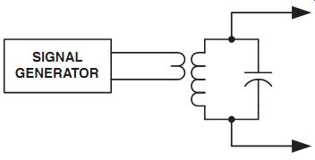
17-4 Two-turn link coupling.
Capacitance and inductance measurements
The Heathkit Model HD-1422 (a noise bridge similar to those mentioned in this section) comes with a calibrated 100-pF silver mica test capacitor (called CTEST in the Heath literature) and a calibrated 4.7-_H test inductor (called LTEST), which are used to measure inductance and capacitance, respectively. The idea is to use the test components to form a series-tuned resonant circuit with an unknown component. If you find the resonant frequency then you can calculate the unknown value. In both cases, the series-tuned circuit is connected across the UNKNOWN terminals of the HD-1422 and the series-tuned procedure is followed.
Inductance
To measure inductance, connect the 100-pF CTEST capacitor in series with the unknown coil across the UNKNOWN terminals of the HD-1422. When the null frequency is found, find the inductance from L _ 253/F2; L is the inductance in micro henrys (uH) and F is the frequency in megahertz.
Capacitance
Connect LTEST across the UNKNOWN terminals in series with the unknown capacitance. Set the RESISTANCE control to zero, tune the receiver to 2 MHz, and readjust the REACTANCE control for null. Without readjusting the noise bridge control connect LTEST in series with the unknown capacitance and retune the receiver for a null. Capacitance can now be calculated from C _ 5389/F2; C is in picofarads and F is in megahertz.