AMAZON multi-meters discounts AMAZON oscilloscope discounts
One of the first things that you learn in radio communications and broadcasting is that antenna impedance must be matched to the transmission line impedance and that the transmission line impedance must be matched to the output impedance of the transmitter. The reason for this requirement is that maximum power transfer between a source and a load always occurs when the system impedances are matched. In other words, more power is transmitted from the system when the load impedance (the antenna), the transmission line impedance, and the transmitter output impedance are all matched to each other.
Of course, the trivial case is where all three sections of the system have the same impedance. For example, an antenna could have a simple 75 ohm resistive feedpoint impedance (typical of a half-wave dipole in free space) and a transmitter with an output impedance that will match 75 ohm . In that case, you only need to connect a 75 ohm standard-impedance length of coaxial cable between the transmitter and the antenna.
Job done! Or so it seems....
But, in other cases, the job is not so simple. In the case of the "standard" antenna, for example, the feedpoint impedance is rarely what the books say it should be. That ubiquitous dipole, for example, is nominally rated at 75 ohm but even the simplest antenna books show that value is an approximation of the theoretical free space impedance. At locations closer to the earth's surface, the impedance could vary over the approximate range of 30 to 130 ohm and it might have a substantial reactive component.
But there is a way out of this situation. You can construct an impedance matching system that will marry the source impedance to the load impedance. This section examines several matching systems that are useful in a number of antenna situations.
Impedance matching approaches
Antenna impedance might contain both reactive and resistive components. In most practical applications, we are searching for a purely resistive impedance (Z=R), but that ideal is rarely achieved. A dipole antenna, for example, has a theoretical free-space impedance of 73 ohm at resonance. But as the frequency applied to the dipole is varied away from resonance, however, a reactive component (_jX) appears.
When the frequency is greater than resonance, then the antenna looks like an inductive reactance so the impedance is Z = R + jX. Similarly, when the frequency is less than the resonance frequency, the antenna looks like a capacitive reactance so the impedance is Z =R + jX. Also, at distances closer to the earth's surface the resistive component might not be exactly 73 ohm, but might vary from about 30 to 130 ohm.
Clearly, whatever impedance coaxial cable is selected to feed the dipole, it stands a good chance of being wrong.
The method used for matching a complex load impedance (such as an antenna) to a resistive source, the most frequently encountered situation in practical radio work, is to interpose a matching network between the load and the source (Fig. 19-1).
The matching network must have an impedance that is the complex conjugate of the complex load impedance. For example, if the load impedance is R _ jX, then the matching network must have an impedance of R _ jX; similarly, if the load is R _ jX, then the matching network must be R _ jX. The sections that follow show some of the more popular networks that accomplish this job.
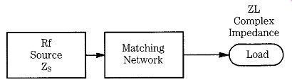
19-1 Block diagram of an antenna impedance-matching scheme.
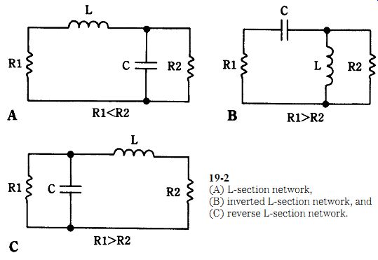
19-2 (A) L- section network, (B) inverted L- section network, and (C) reverse
L- section network.
L- section network
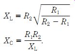
The L- section network is one of the most used, or at least most published, antenna-matching networks in existence: it rivals even the pi-network. A circuit for the L- section network is shown in Fig. 19-2A. The two resistors represent the source (R1) and load (R2) impedances. The elementary assumption of this network is that R1 _ R2. The design equations are:
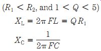
(19-1)

(19-2)
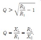
(19-3)

(19-4)
You will probably most often see this network published in conjunction with less than-quarter-wavelength long-wire antennas. One common fault of those books and articles is that they typically call for a "good ground" in order to make the antenna work properly. But they don't tell you what a "good ground" is and how you can obtain it. Unfortunately, at most locations a good ground means burying a lot of cop per conductor-something that most of us cannot afford. In addition, often the person who is forced to use a long-wire instead of a better antenna cannot construct a "good ground" under any circumstances because of landlords and/or logistics problems.
The very factors that prompt the use of a longwire antenna in the first place also prohibit any form of practically obtainable "good ground." But there is a way out: radials. A good ground can be simulated with a counterpoise ground constructed of quarter-wavelength radials. These radials have a length in feet equal to 246/FMHz, and as few as two of them will work wonders.
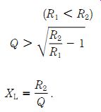
Another form of L-section network is shown in Figure 19-2B. This circuit differs from the previous circuit in that the roles of the L and C components are reversed.
As you might suspect, this role reversal brings about a reversal of the impedance relationships: in this circuit, the assumption is that driving source impedance R1 is larger than load impedance R2 (i.e., R1 _ R2). The equations are:
(19-5)

(19-6)
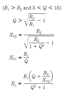
Still another form of L- section network is shown in Figure 19-2C. Again, we are assuming that the driving source impedance, R1, is larger than load impedance, R2 (i.e., R1 _ R2). In this circuit, the elements are arranged similarly to those in Figure 19-2A, with the exception that the capacitor is at the input, rather than the output, of the network. The equations governing this network are:
(19-7)

(19-8)

(19-9)

(19-10)
Thus far, only matching networks that are based on inductor and capacitor circuits have been considered. Also, transmission-line segments can be used as impedance-matching devices. Two basic forms are available: quarter-wave sections and series-matching section.
Pi- (_) networks
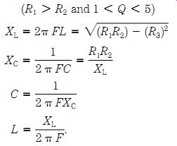
The pi-network shown in Fig. 19-3 is used to match a high source impedance to a low load impedance. These circuits are typically used in vacuum-tube RF power amplifiers that need to match low antenna impedances. The name of the circuit comes from its resemblance to the greek letter "pi" (_). The equations for the pi network are:
(19-11)

(19-12)

(19-13)

(19-14)
19-3 Pi- (_) network.
Split-capacitor network
The split capacitor network shown in Fig. 19-4 is used to transform a source impedance that is less than the load impedance. In addition to matching antennas, this circuit is also used for interstage impedance matching inside communications equipment. The equations for design are:
(19-15)

(19-16)
19-4 Split-capacitor network.
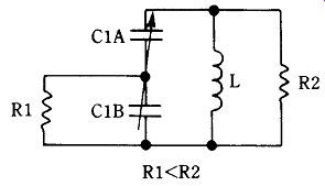
Transmatch circuit
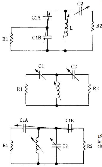
One version of the transmatch is shown in Fig. 19-5. This circuit is basically a combination of the split-capacitor network and an output tuning capacitor (C2). For the HF bands, the capacitors are on the order of 150 pF per section for C1 and 250 pF for C2. The roller inductor should be 28 H. The transmatch is essentially a coax-to-coax impedance matcher and is used to trim the mismatch from a line be fore it affects the transmitter.
Perhaps the most common form of transmatch circuit is the tee-network shown in Fig. 19-6. This network is lower in cost than some of the others, but suffers a problem. Although it does, in fact, match impedance (and thereby, in a naive sense, "tunes out" VSWR on coaxial lines), it also suffers a high-pass characteristic. This network, therefore, does not reduce the harmonic output of the transmitter. The simple tee-network does not serve one of the main purposes of the antenna tuner: harmonic reduction. An alternative network, called the SPC transmatch, is shown in Fig. 19-7. This version of the circuit offers harmonic attenuation as well as matching impedance.
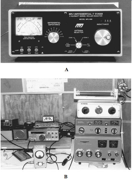
Figure 19-8 shows commercially available antenna tuners based on the transmatch design. The unit shown in Fig. 19-8A is manufactured by MFJ. It contains the usual three tuning controls, here labeled Transmitter, Antenna, and Inductor.
Included in this instrument is an antenna selector switch that allows the operator to select a coax cable antenna through the tuner to connect input to output (coax) without regard to the tuner and select a balanced antenna or an internal dummy load. The instrument also contains a multifunction meter that can measure 200 or 2000 W (full-scale) in either forward or reverse directions. In addition, the meter operates as a VSWR meter.
Figures 19-8 shows a tuner from the United Kingdom. This instrument, the Nevada model, is low-cost but contains the three basic controls. For proper operation, an external RF power meter or VSWR meter is required. This tuner and a Heathkit transmatch antenna tuner are shown in Fig. 19-8B. There are SO-239 coaxial connectors for input and unbalanced output along with a pair of posts for the parallel line output. A three-post panel is used to select which antenna the RF goes to: unbalanced (coax) or parallel. The roller inductor is in the center and it allows the user to set the tuner to a wide range of impedances over the entire 3- to 30-MHz HF band.
19-5 Transmatch network.
19-6 Tee-network.
19-7 Improved SPC transmatch circuit.
19-8 Commercial HF antenna-matching networks.
Coaxial cable balun transformers
A balun is a transformer that matches an unbalanced resistive source impedance (such as a coaxial cable) and a balanced load (such as a dipole antenna). With the circuit of Fig. 19-9, you can make a balun that will transform impedance at a 4:1 ratio, with R2 = 4 x R1. The length of the balun section coaxial cable is:

(19-17)
where
Lft =the length in feet
V = the velocity factor of the coaxial cable (a decimal fraction)
F_MHz = the operating frequency in megahertz.
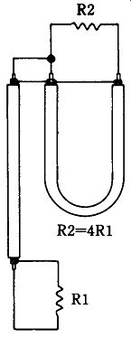
19-9 Coaxial balun transformer.
Matching stubs
A shorted stub can be built to produce almost any value of reactance. This can be used to make an impedance-matching device that cancels the reactive portion of a complex impedance. If you have an impedance of, for example, Z = R + j30 ohm, you need to make a stub with a reactance of - j30 ohm to match it. Two forms of matching stubs are shown in Figs. 19-10A and 19-10B. These stubs are connected exactly at the feedpoint of the complex load impedance, although they are sometimes placed further back on the line at a (perhaps) more convenient point. In that case, however, the reactance required will be transformed by the transmission line between the load and the stub.
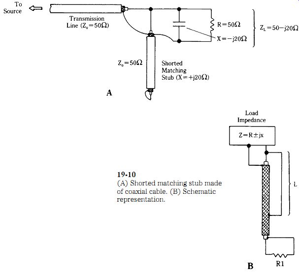
19-10 (A) Shorted matching stub made of coaxial cable. (B) Schematic representation.
Quarter-wavelength matching sections
Figure 19-11 shows the elementary quarter-wavelength transformer section connected between the transmission line and the antenna load. This transformer is also sometimes called a Q- section. When designed correctly, this transmission-line transformer is capable of matching the normal feedline impedance (ZS) to the antenna feedpoint impedance (ZR). The key factor is to have available a piece of transmission line that has an impedance Zo of:

(19-18)
Most texts show this circuit for use with coaxial cable. Although it is certainly possible and even practical in some cases, for the most part, there is a serious flaw in using coax for this project. It seems that the normal range of antenna feedpoint impedances, coupled with the rigidly fixed values of coaxial-cable surge impedance available on the market, combines to yield unavailable values of Zo. Although there are certainly situations that yield to this requirement, many times the quarter-wave section is not usable on coaxial-cable antenna systems using standard impedance values.
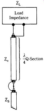
19-11 Quarter-wavelength Q- section impedance transformer.
On parallel transmission-line systems, on the other hand, it is quite easy to achieve the correct impedance for the matching section. Use Eq.(19-18) to find a value for Zo then calculate the dimensions of the parallel feeders. Because you know the impedance, and can more often than not select the conductor diameter from avail able wire supplies, you can use the following equation to calculate conductor spacing:

(19-19)
...where...
S _ the spacing
D_ the conductor diameter (D and S in the same units)
Z _ the desired surge impedance.
From there we can calculate the length of the quarter-wave section from the familiar 246/FMHz.
Series-matching section
The quarter-wavelength section discussed above suffers from several draw backs: it must be located at the antenna feedpoint, it must be a quarter-wavelength, and it must use a specified (often nonstandard) value of impedance. The series matching section is a generalized case of the same idea and permits us to build an impedance transformer that overcomes most of these faults. According to The ARRL Antenna Book, this form of transformer is capable of matching any load resistance between about 5 and 1200 ohm. In addition, the transformer section is not located at the antenna feedpoint.
Figure 19-12 shows the basic form of the series-matching section. There are three lengths of coaxial cable: L1, L2, and the line to the transmitter. Length L1 and the line to the transmitter (which is any convenient length) have the same characteristic impedance, usually 75 ohm . Section L2 has a different impedance from L1 and the line to the transmitter, usually 75 ohm . Notice that only standard, easily obtainable values of impedance are used here.
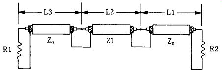
19-12 Matching- section impedance transformer.
The design of this transformer consists of finding the correct lengths for L1 and L2. You must know the characteristic impedance of the two lines (50 and 75 ohm are given as examples) and the complex antenna impedance. If the antenna is non resonant, this impedance is of the form: Z _ R _ jX, where R is the resistive portion, X is the reactive portion (inductive or capacitive) and j is the so-called "imaginary" operator (i.e., ). If the antenna is resonant, then X _ 0 and the impedance is simply R.
The first chore in designing the transformer is to normalize the impedances:
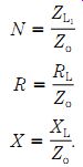
(19-20)

(19-21)

(19-22)
The lengths are determined in electrical degrees, and from that determination you can find length in feet or meters. If you adopt ARRL notation and define A _ tan (L1), and B _ tan (L2) then the following equations can be written:
If
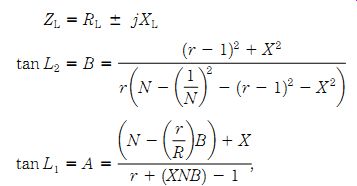
(19-23)

(19-24)

(19-25)
(19-26)

(19-27)

(19-28)

(19-29)
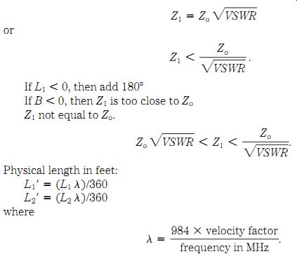
The physical length is determined from arctan (A) and arctan (B) divided by 360 and multiplied by the wavelength along the line and the velocity factor. Although the sign of B might be selected as either _ or _, the use of _ is preferred because a shorter section is obtained. In the event that the sign of A turns out negative, add 180 degrees to the result.
There are constraints on the design of this transformer. The impedances of the two sections (L1 and L2) cannot be too close together. In general, the following relationships must be observed:
Either
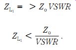
(19-30)
or

(19-31)