AMAZON multi-meters discounts AMAZON oscilloscope discounts
Filters are frequency-selective circuits that pass some frequencies and reject others.
Filters are available in several different flavors: low-pass, high-pass, bandpass, and notch. All of these filters are classified according to the frequencies that they pass (or reject). The breakpoint between the accept band and the reject band is usually taken to be the frequency at which the passband response falls off -3 dB. The four different types are characterized below.
Low-pass filters pass all frequencies below the cutoff frequency defined by the -3-dB point (Fig. 23-1A). These filters are useful for removing the harmonic content of signals or eliminating interfering signals above the cutoff frequency.
High-pass filters pass all frequencies above the -3-dB cutoff point (Fig. 23-1B).
These filters are useful for eliminating interference from strong signals below the cutoff point. For example, a person using a shortwave receiver might wish to install a 1800-kHz high-pass filter to eliminate signals from strong AM broadcast stations.
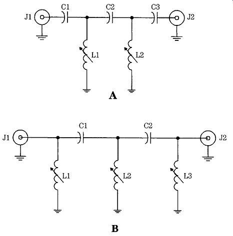
Bandpass filters pass all frequencies between lower (FL) and upper (FH) -3-dB points, while rejecting those outside the FH-FL range. Bandpass filters are either wideband (low Q) or narrow band (high Q), as shown in Fig. 23-1C and 23-1D, respectively.
Q is the quality factor of the bandpass filter and is defined as the ratio of the center frequency to the bandwidth. For example, if a filter is centered on 10,000 kHz, and it has a 25-kHz bandwidth between the lower and upper -3-dB points, then the Q is 10,000/25 = 400.
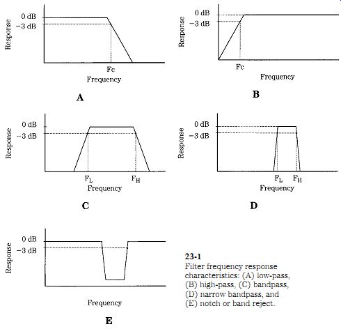
23-1 Filter frequency response characteristics: (A) low-pass, (B) high-pass,
(C) bandpass, (D) narrow bandpass, and (E) notch or band reject.
Notch filters (band reject filters), pass all frequencies except those between lower and upper cutoff frequencies (Fig. 23-1E). Some notch filters are made broad, but many are very narrow. The latter are designed to suppress a single frequency. For example, a local FM broadcast signal will often interfere with television or two-way radio services. A notch filter tuned to that frequency will wipe it out. Similarly, on an AM band receiver, if it is being desensitized by a strong local station, reducing reception of all other frequencies on the AM band, a single-frequency notch filter can be used to suppress that one station's signal, leaving the other frequencies untouched.
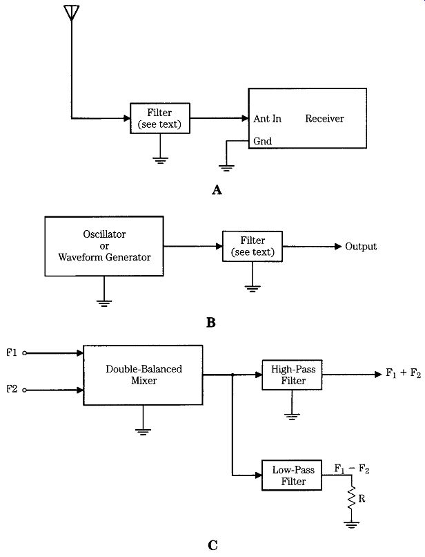
23-2 Filter applications: (A) ahead of a receiver antenna input to reduce
unwanted signals, (B) at the output of oscillators and other waveform generators,
(C) at the output of a double balanced mixer in a diplexer impedance-matching
circuit.
Filter applications
Figure 23-2 shows several different types of filter applications. In Fig. 23-2A, the filter is placed between the antenna and the antenna input of a receiver. Its function is to remove unwanted signals before they reach the front end. Whether a high-pass, low-pass, or bandpass filter is used depends on the local situation (i.e., the frequencies that you wish to eliminate).
There are several good reasons for using a filter ahead of a receiver, even when the strong local signal is not within the normal passband of the receiver. The narrow passband selectivity of the receiver is set in the IF amplifiers and the RF ("front end") selectivity is a lot broader. As a result, strong signals often reach the input stage, which will be either an RF amplifier or mixer. In either case, the unwanted signal can drive the input of the receiver into a nonlinear region of operating, creating either harmonics or intermodulation distortion products. These spurious signals not only are audible in the receiver (in some combinations), but also take up part of the receiver's dynamic range.
Figure 23-2B shows a filter placed at the output of an oscillator circuit. If the output signal is a pure sine wave, it will contain only one frequency (i.e., the desired oscillation frequency). But if there is even a little distortion, then harmonics will be present. These harmonics will adversely affect some circuits that the oscillator drives, so they must be eliminated.
The most usual filter used on oscillator outputs is the low-pass filter. The filter is designed with a cutoff frequency that is between the desired fundamental frequency and its second harmonic.
Another type of filter is a very high-Q bandpass filter. These filters are very narrow. The purpose of using such a filter is to reduce the phase noise on the oscillator signal. It takes a very narrow-band filter to do this trick, and both the oscillator frequency and the passband of the filter must be stable or the poly will be unsuccessful.
The circuit in Fig. 23-2C shows the use of two filters at the output of a double balanced mixer (DBM). The DBM receives two input frequencies, F1 and F2, and will output a spectrum of mF1 _ nF2, where m and n are integers greater than 1 (on non-DBM mixers, m and n might be 1, indicating that F1, F2, or both may appear in the output). It is not sufficient to pick off the signal in the desired band and reject the signals in the unwanted band. Those unwanted signals will be reflected back into the mixer and might adversely affect its operation. The proper strategy is to use a circuit that passes the undesired signals to a dummy load that has a resistance equal to the mixer output impedance. This arrangement allows the dummy load to absorb the unwanted signals rather than permits them to reflect back into the mixer circuit.
Filter construction
A filter must be constructed properly if it is to work correctly. The two main factors to consider are layout and shielding.
Proper layout involves two main issues. First, keep the output and input ends of the circuit physically separated so as to prevent coupling of signal energy between them. Second, make sure that all inductors in the filter are shielded, arranged at right angles to each other, or wound on toroidal cores. All three of these approaches are used because they reduce coupling between inductors. Shielding keeps the magnetic field of the coil contained within the metallic shield. When cylindrical, solenoid-wound coils (i.e., those with a length greater than the diameter) are placed at right angles with respect to each other then magnetic coupling is minimized. A toroidal coil form is doughnut shaped and it naturally contains the magnetic field because of its geometry.
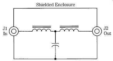
23-3 Filter success often depends on layout and construction. Shielded enclosures
are a must!
Shielding of the entire filter circuit is necessary to keep outside signal energy from getting into the filter and to ensure that the only signal reaching the load (i.e., the circuit being driven by the filter) has passed through the filter circuit. Figure 23-3 shows a sample filter (such as those covered in this section) enclosed within a shielded box. The signal input and output jacks. (J1 and J2) are coaxial connectors.
The box should be either a die-cast aluminum box with a tight-fitting lid (some brands are pretty sloppy, so be careful), a sheet-metal aluminum box with overlap ping lips for a RF seal, or a box specifically intended for RF work (these can be identified by the RF "finger" gaskets around the edge of the cover).
Filter design approach
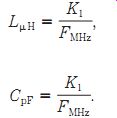
The design of inductor-capacitor (LC) filters for radio frequency (RF) circuits is often presented in its most arcane mathematical form. Use of that design approach allows you to optimize designs. However, this form is also above the capabilities of many people who could put filters to good use. A different approach is needed, and that approach is the normalized 1-MHz model. In this design approach, a model is built by calculating the component values for 1 MHz. The component values can be scaled for any frequency by dividing the 1-MHz value by the desired frequency, expressed in megahertz.
A limitation on this approach is that it assumes that the input and output impedances are both equal to 50-ohm (i.e., the design impedance of the 1-MHz model filter). Because RF systems tend to have 50-ohm impedances; however, this restriction does not pose a big problem in most cases.
Low-pass filters
Low-pass LC filters are recognized by having the inductor (or inductors) in series with the signal path and the capacitors shunted across the signal path. The low pass filter (LPF) attenuates all signal frequencies above its cutoff and passes all frequencies below the cutoff.
Figure 23-4 shows two basic single- section LPFs. The t-filter configuration is shown in Fig. 23-4A, and the pi-filter configuration is shown in Fig. 23-4B. The values of the capacitors and inductors are calculated using the equations:
(23-1)

(23-2)
23-4 (A) Three-element, T- section low-pass filter and (B) three-element
pi- section low-pass filter.
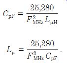
These equations will also be used to calculate the values of the components in the other filters as well, although the numbering of the constants (K) will be different. The values of constants K1 and K2 are found from Table 23-1.
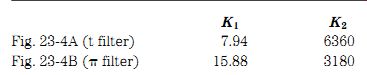
Table 23-1. Filter design constants for Fig. 23-4
Example: Calculate the component values for both t-filter and pi-filter configurations for a low-pass filter with a cut-off frequency of 35 MHz.
t filter:
CpF _ 6360_35 _ 182 pF
CpF _ K2uFMHz
L_H _ 7.94_35 _ 0.27_H
L_H _ K1uFMHz
The inductors can be either home-wound or purchased. Although it's possible to use adjustable inductances and capacitances in these filter circuits, it is not recommended that they be adjusted in the circuit. The adjustable components can allow one to obtain the specific values called for in the equations, but they should be preset to the value prior to being connected into the circuit. This job can be done using either a LC bridge or a digital LC meter, such as are found on some digital multi meters.
The inductors should be single components, wound, or selected and set for the specific inductance required. The capacitors, on the other hand, can be made up from several capacitors in series and parallel in order to obtain the correct value. Re member when doing this, however, that tolerances can make the whole thing less than useful. Most capacitors have tolerances of 5 or 10%, unless otherwise noted. It is best to use as close a value capacitor as possible, and that could involve hand selecting capacitors, according to actual capacitance using a meter or bridge.
Each section of the filter provides a certain degree of attenuation, as indicated by the steepness of the roll-off slope beyond the cutoff frequency. Cascading sections will increase the roll-off slope, so they will also increase the attenuation obtained at any given frequency in the stopband. Figure 23-5 shows t-filter and pi filter circuit in the two- section version. The calculation constants are shown in Table 23-2.
High-pass filters
A high-pass filter (HPF) attenuates signal frequencies below the _3-dB cutoff frequency and passes signal frequencies above the cutoff frequency.
Single- section high-pass filters are shown in Figs. 23-6A and 23-6B. These are the inverse of the LPF single- section filters in that the capacitors are in series with the signal path, and the inductors are across the signal path. The version in Fig. 23-6A is the t-filter configuration, and that in Fig. 23-6B is the pi-filter. The values for the components are found in Table 23-3.
_ filter:
CpF _ 3180_35 _ 91 pF.
CpF _ K2 uFMHz
L_H _ 15.88_35 _ 0.454_H
L_H _ k1uFMHz
Example: Find the component values for a single- section high-pass filter with a cutoff frequency of 40 MHz.
t filter
(Fig. 23-6A):
L1 _ 3.97_40 _ 0.1_H
L1 _ KL1uFMHz ,
_ filter
(Fig. 23-6B):
C1 _ 1590 degree 40 _ 40 pF.
C1 _ KC1uFMHz L1 _ 7.94_40 _ 0.2_H L1 _ KL1uFMHz C1 _ 3180_40 _ 79.5 pF C1 _ KC1uFMHz
Two section high-pass filters are shown in Figs. 23-7A (t-filter) and 7B (pi-filter), and the 1-MHz model constants are shown in Table 23-4.
23-5 (A) Five-element, T- section low-pass filter and (B) five-element, pi- section low pass filter.
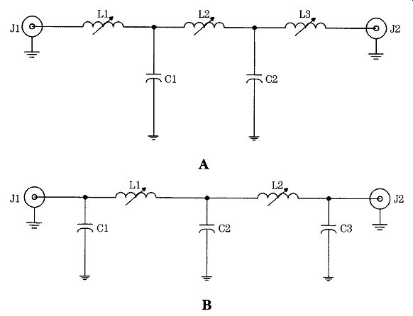
Table 23-2. Filter design constants for Fig. 23-5.
23-6 (A) Three-element, T- section high-pass filter and (B) three-element,
pi-section high pass filter.

Table 23-3. Filter design constants for Fig. 23-6
23-7 (A) Five-element, T- section high-pass filter and (B) five element,
pi- section high-pass filter.

Table 23-4. Filter design constants for Fig. 23-7
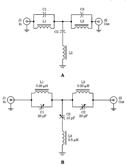
Bandpass filters
A bandpass filter passes only those frequencies between lower and upper _3-dB cutoff frequencies and attenuates all others. One simple way to obtain a bandpass frequency response characteristic is to cascade low-pass and high-pass sections (Fig. 23-8). The LPF is designed with a cutoff frequency equal to the high cutoff frequency in the passband, and the HPF is designed to cutoff at the low point in the de sired passband. The values are as calculated for the individual sections.
23-8 Bandpass filter made by cascading low-pass and high-pass sections.
23-9 AM BCB (500 to 2000 kHz) bandpass filter.
Enhancing AM band reception
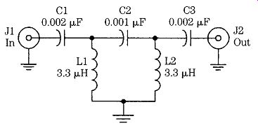
Figure 23-9 shows a bandpass filter for the AM broadcast band. This type of filter can be used between the antenna and antenna input of an AM broadcast band receiver in order to reduce any out-of-band signals that might interfere with reception or reduce the performance of the receiver. This filter consists of a 2000-kHz low-pass filter cascaded with a 500-kHz high-pass filter.
Removing the AM band
Many shortwave receivers are afflicted with a marginal front end-even though the rest of the receiver is pretty decent. For example, sensitivity and IF selectivity might be real good, but if the third-order intercept point, dynamic range, and inter modulation performance of the receiver aren't up to snuff then the receiver is likely to overload, desensitize, or hear signals that aren't really there.
One of the principal sources of front-end overload is local AM band signals. The broadcasters tend to be very local (i.e., down the block or less than a mile away for many listeners) and very strong. Although a 1000-W station might not impress any one in the 25-m shortwave band, it can have a very large local field strength two blocks away. And the 50,000-W clear-channel "blowtorches" really raise havoc. The signal need not be in the same band, or near the same frequency, as you are trying to tune in to. The front ends of a lot of receivers, even in relatively expensive receivers, can be marginal enough that strong signals will get past the tuning or filtering to affect the operation of the input amplifier or mixer stage.
The only cure for the problem is to eliminate the offending signals. In other words, place a high-pass filter ahead of the receiver that will attenuate the AM signals, but pass all higher frequencies. All frequencies below 2000 kHz are severely attenuated in these filters, so the offending AM signals will be reduced considerably.
Figure 23-10A is a high-pass filter with a cutoff frequency of about 1800 kHz.
This is a classic five-element, T- section high-pass filter. It is identified as a high-pass filter because the capacitors are in series with the signal line and the inductors are shunted across the signal line (a low-pass filter reverses these). This filter can be built using ordinary NPO disk ceramic capacitors for C1, C2, and C3. Alternatively, silver-mica units can be used. To obtain the 2000-pF value in silver mica, it might be necessary to parallel two 1000-pF units. The 3.3-uH coils can be "store-bought" or wound on toroid core forms. Two popular forms for this particular application are the T-50-2 (red) and T-50-15 (red/white) cores. The AL value for the T-50-2 (red) is 49 and for the T-50-15 (red/white) is 135. These values translate to 26 turns of wire for the T-50-2 (red) and 17 turns for the T-50-15 (red/white).
Another variant is shown in Fig. 23-10B. This circuit uses a 977-kHz mid-band suppression feature, consisting of two series-resonant circuits (C4/L1 and C5/L2), along with the normal configuration of series capacitors (C1, C2, and C3). Still another variation is shown in Fig. 23-10C. This filter has a slightly lower -3-dB cutoff frequency (i.e., 1600 kHz, but it is capable of a higher degree of attenuation than the previous filters, especially close to the cutoff frequency; e.g., at the second harmonic of the cutoff frequency).
This filter provides up to -40 dB of suppression. Notice, however, that maintaining the theoretical suppression depends in part on good layout and construction practices. Each section of the filter should be enclosed in its own shielded compartment of a well-made shielded enclosure; coaxial input and output connectors are used at J1 and J2.
Notice in Fig. 23-10C that the capacitance values are nonstandard. These capacitances can be approximated by standard capacitance values if two or more capacitors are placed in either series or parallel, as needed. Try various combinations until the closest fit is obtained. A much closer fit can then be achieved by measuring the actual capacitance of capacitors proposed for use in the circuit. All capacitors have a tolerance on the nominal value, so the actual value is different from the marked value by a small amount.
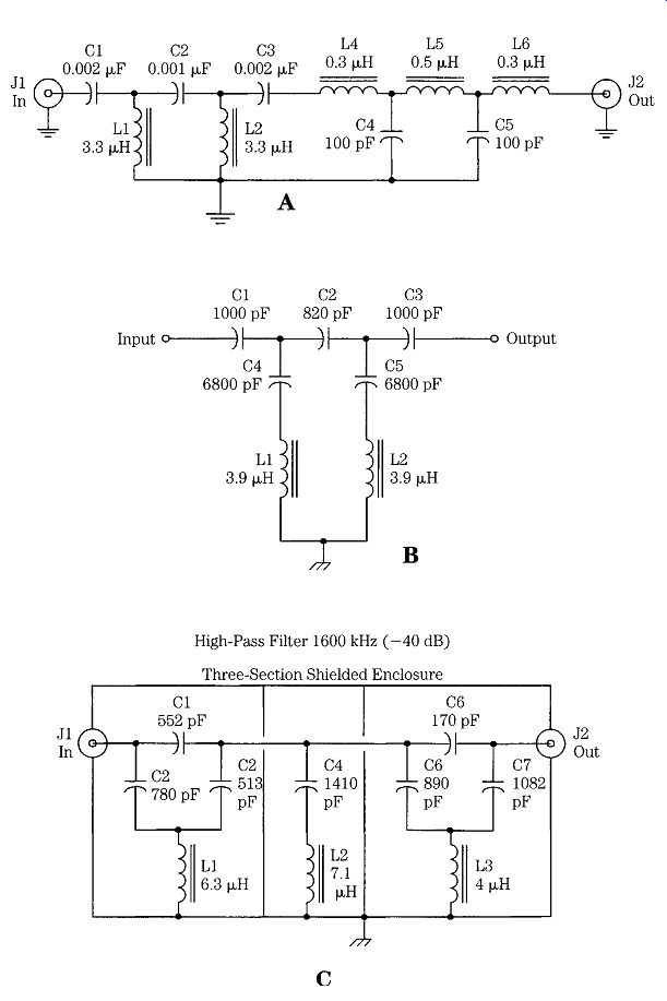
23-10 High-pass AM band suppression filters (A) using the five-element,
T- section design, (B) with mid-band suppression, and (C) AM band "Thunder
Lizard" filter.
Notch filters
A notch filter is a breed of bandstop filter with a high Q (i.e., a narrow band width). They are designed to attenuate a single frequency or, actually, a narrow band of frequencies around a single center frequency.
Notch filters can be used to attenuate a single offending signal. For example, if you live near a FM broadcaster, you might notice that the signal is spread over a wide area of the band or that it appears at several spots on the band. Although this could be the result of a FM broadcaster's transmitter in need of repair, it's much more likely caused by spurious response of your receiver from front-end overload.
Two basic ways are used to notch out a single frequency, although they are often combined for improved effectiveness. A parallel-resonant trap (Fig. 23-11A) has an impedance that is very high at the resonant frequency and very low at frequencies removed from resonance. A parallel-resonant trap placed in series with the signal path will, therefore, severely attenuate frequencies at or near its resonant frequency and pass all others. A series-resonant trap (Fig. 23-11B) is just the opposite: it has a very low impedance at its resonant frequency and a high impedance at all other frequencies. A series-resonant trap shunted across should attenuate signals at or close to the resonant frequency.
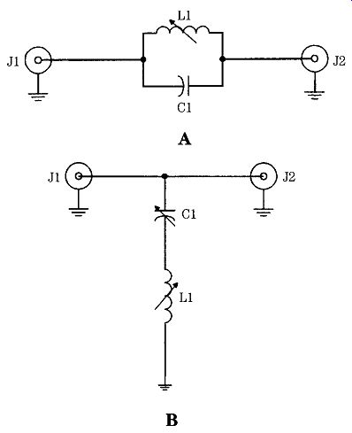
23-11 Notch filters/wave-traps: (A) parallel resonant in series with the
signal path and (B) series resonant in parallel with the signal path.
The resonant frequency is found from:

...(23-3) ... where F is in megahertz (MHz) L is in microhenrys (uH) C is
in picofarads (pF).
In the practical sense, this equation is not too terribly useful because the better approach is to select a trial value for either inductance or capacitance (depending on which is more convenient) and then calculate the required value for the other component. These equations are:
(23-4) or (23-5)
The parallel- and series-resonant circuits can be connected together to form a multi section notch filter (Fig. 23-12A). Indeed, this is the approach normally taken in commercial wavetrap circuits. The capacitances shunted across L1 and L3 are shown as two units in parallel to indicate that it will probably be necessary to make special, nonstandard values from two or more capacitors.
A multi section notch filter for the FM broadcast band is shown in Fig. 23-12B.
This type of circuit is often sold in video stores as a "FM wave trap," and it is used to eliminate FM "herringbone" interference patterns on VHF television receivers. This filter consists of three filter sections in cascade: two parallel-resonant filters sandwiching a series-resonant filter between them.
One other form of notch filter can be used especially at VHF frequencies, al though in theory it would work from dc to daylight. A transmission line will reflect its terminating impedance every half wavelength back down the line. Thus, if the end of a transmission line is short-circuited then the 0-ohm impedance will appear at points every half wavelength back toward the source from the short. This fact makes it possible to use a half-wavelength shorted transmission line stub as a notch filter; both coaxial cable and twin-lead can be used in this capacity (Fig. 23-13).
23-12 (A) Multi section notch filter design and (B) multi section notch
filter for the FM BCB.
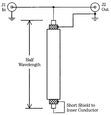
23-13 Use of a half-wavelength shorted stub across the signal line to attenuate
a single-frequency signal.
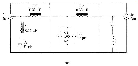
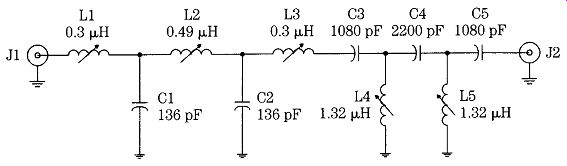
23-14 A 2- to 33-MHz bandpass filter.
The length of the transmission line is the physical half-wavelength for the design frequency multiplied by the velocity factor of the transmission line. The velocity factor is a decimal number between 0 and 1 that indicates the speed of signal propagation in the line as a fraction of the speed of light:

(23-6)
For example, suppose you need a half-wave shorted stub to remove a 100-MHz FM broadcast signal. The available coaxial cable is polyfoam cable with a velocity factor of 0.82; the length is:

(23-7)

(23-8)
In actual operation, the required length might be a little different, and the correct length must be found from experimentation. The reason is that the actual velocity factor might not be exactly as published and the length measurement will have a certain error. As a result, it's usually good practice to cut the trial length a few centimeters too long and then use trial and error to find the actual correct length. I've used a pin through the coax as a shorting bar to do the experimental trials, and it seemed to work well.
More on bandpass filters
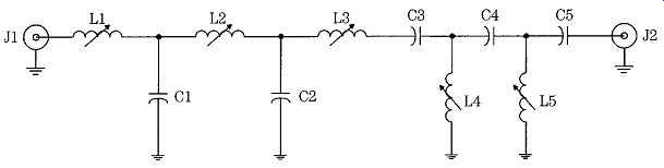
A bandpass filter is designed to pass all frequencies that are above a lower cutoff frequency and all frequencies that are below an upper cutoff frequency. Figures 23-14 and 23-15 show two approaches to making a bandpass filter for the high-frequency (HF) shortwave bands. The circuit in Fig. 23-14 is designed for a frequency band of 2 to 33 MHz, so it will encompass the entire HF shortwave band while eliminating interference from LF and MW AM band broadcasters as well as VHF stations. Notice that each section is built inside its own shielded compartment. This is good layout practice for any multi section filter and it prevents interaction between the elements (especially coils).
The bandpass filter in Fig. 23-15 is not so elegant as the previous example but it serves the purpose. This approach to bandpass filter design cascades low-pass and high-pass sections. The input side of Fig. 23-15 is the AM BCB filter used in the last paragraph and the output section is a 33-MHz low-pass filter of similar design.
23-15 A 2- to 33-MHz bandpass filter based on cascading low-pass and high-pass
sections.
Conclusion
Although RF filters involving LC elements are often presented as a difficult subject (which it is!), simplifications are possible using normalized 1-MHz models and a little arithmetic. The filters in this section are not necessarily optimized, but they will turn in more than merely adequate performance if you are diligent when constructing them.