AMAZON multi-meters discounts AMAZON oscilloscope discounts
The mathematics of transmission lines, and certain other devices, becomes cumber some at times, especially when dealing with complex impedances and "nonstandard" situations. In 1939, Philip H. Smith published a graphical device for solving these problems, followed in 1945 by an improved version of the chart. That graphic aid, somewhat modified over time, is still in constant use in microwave electronics and other fields where complex impedances and transmission line problems are found.
The Smith chart is indeed a powerful tool for the RF designer.
Smith chart components
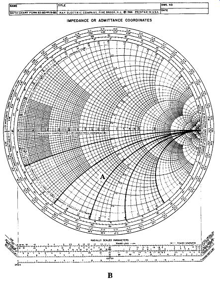
The modern Smith chart is shown in Fig. 26-1 and consists of a series of over lapping orthogonal circles (i.e., circles that intersect each other at right angles). This section will dissect the Smith chart so that the origin and use of these circles is apparent. The set of orthogonal circles makes up the basic structure of the Smith chart.
The normalized impedance line
A baseline is highlighted in Fig. 26-2 and it bisects the Smith chart outer circle.
This line is called the pure resistance line, and it forms the reference for measurements made on the chart. Recall that a complex impedance contains both resistance and reactance and is expressed in the mathematical form:

(26-1)
where .......
Z = the complex impedance
R = the resistive component of the impedance
X = the reactive component of the impedance
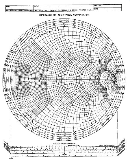
26-1 The Smith chart.
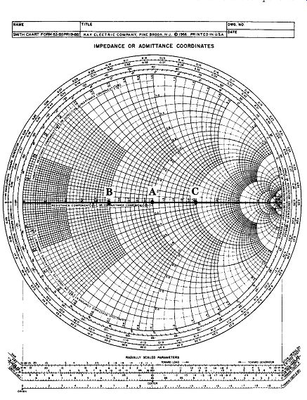
26-2 Normalized impedance line.
The pure resistance line represents the situation where X _ 0 and the impedance is therefore equal to the resistive component only. In order to make the Smith chart universal, the impedances along the pure resistance line are normalized with reference to system impedance (e.g., Zo in transmission lines); for most microwave RF systems the system impedance is standardized at 50-ohm . To normalize the actual impedance, divide it by the system impedance. For example, if the load impedance of a transmission line is ZL and the characteristic impedance of the line is Zo then Z _ ZL /Zo. In other words:

(26-2)
The pure resistance line is structured such that the system standard impedance is in the center of the chart and has a normalized value of 1.0 (see point "A" in Fig. 26-2).
This value derives from Zo/Zo_ 1.0.
To the left of the 1.0 point are decimal fraction values used to denote impedances less than the system impedance. For example, in a 50-ohm transmission-line system with a 25-ohm load impedance, the normalized value of impedance is 25 ohm/50-ohm or 0.50 ("B" in Fig. 26-2). Similarly, points to the right of 1.0 are greater than 1 and denote impedances that are higher than the system impedance. For example, in a 50-ohm sys tem connected to a 100-ohm resistive load, the normalized impedance is 100 ohm/50-ohm , or 2.0: this value is shown as point "C" in Fig. 26-2. By using normalized impedances, you can use the Smith chart for almost any practical combination of system and load and/or source impedances, whether resistive, reactive, or complex.
Reconversion of the normalized impedance to actual impedance values is done by multiplying the normalized impedance by the system impedance. For example, if the resistive component of a normalized impedance is 0.45 then the actual impedance is:

(26-3)

(26-4)

(26-5)
The constant resistance circles The iso-resistance circles, also called the constant resistance circles, represent points of equal resistance. Several of these circles are shown highlighted in Fig. 26-3.
These circles are all tangent to the point at the righthand extreme of the pure resistance line and are bisected by that line. When you construct complex impedances (for which X _ nonzero) on the Smith chart, the points on these circles will all have the same resistive component. Circle "A," for example, passes through the center of the chart, so it has a normalized constant resistance of 1.0. Notice that impedances that are pure resistances (i.e., Z _ R _ j0) will fall at the inter section of a constant resistance circle and the pure resistance line and complex impedances (i.e., X not equal to zero) will appear at any other points on the circle. In Fig. 26-2, circle "A" passes through the center of the chart so it represents all points on the chart with a normalized resistance of 1.0. This particular circle is sometimes called the unity resistance circle.
The constant reactance circles Constant reactance circles are highlighted in Fig. 26-4. The circles (or circle segments) above the pure resistance line (Fig. 26-4A) represent the inductive reactance (_X ) and the circles (or segments) below the pure resistance line (Fig. 26-4B) represent capacitive reactance (_X). In both cases, circle "A" rep resents a normalized reactance of 0.80. One of the outer circles (i.e., circle "A" in Fig. 26-4C) is called the pure reactance circle.
Points along circle "A" represent reactance only; in other words, an impedance of Z _ 0 _ jX (R _ 0). Figure 26-4D shows how to plot impedance and admittance on the Smith chart. Consider an example in which system impedance Zo is 50-ohm and the load impedance is ZL _ 95 _ j55 _. This load impedance is normalized to:

(26-6)

(26-7)

(26-8)
An impedance radius is constructed by drawing a line from the point represented by the normalized load impedance. 1.9 _j1.1, to the point represented by the normalized system impedance (1.0) in the center of the chart. A circle is constructed from this radius and is called the VSWR circle.
Admittance is the reciprocal of impedance, so it is found from:

(26-9)
Because impedances in transmission lines are rarely pure resistive, but rather contain a reactive component also, impedances are expressed using complex notation:
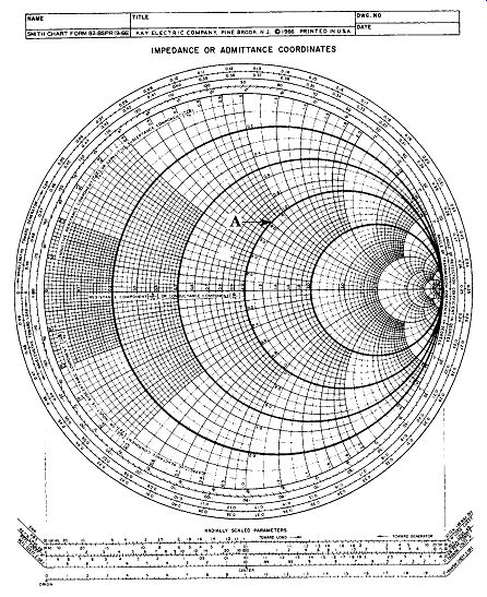
26-3 Constant resistance circles.
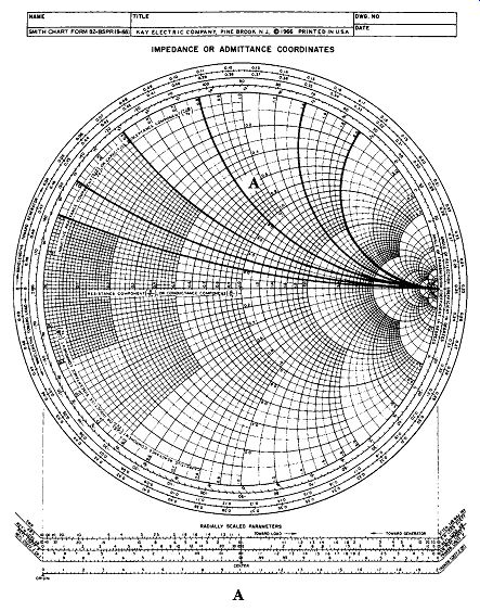
26-4 (A) Constant inductive reactance lines, (B) constant capacitive reactance
lines, (C) angle of transmission coefficient circle, and (D) VSWR circles.
26-4 Continued.

(26-10)
where.....
Z = the complex impedance
R =the resistive component
X = the reactive component.
To find the complex admittance, take the reciprocal of the complex impedance by multiplying the simple reciprocal by the complex conjugate of the impedance. For example, when the normalized impedance is 1.9 + j1.1, the normalized admittance will be:

(26-11)
(26-12)

(26-13)
(26-14)
One of the delights of the Smith chart is that this calculation is reduced to a quick graphical interpretation! Simply extend the impedance radius through the 1.0 center point until it intersects the VSWR circle again. This point of inter section rep resents the normalized admittance of the load.
Outer circle parameters
The standard Smith chart shown in Fig. 26-4C contains three concentric calibrated circles on the outer perimeter of the chart. Circle "A" has already been covered and it is the pure reactance circle. The other two circles define the wavelength distance ("B") relative to either the load or generator end of the transmission line and either the transmission or reflection coefficient angle in degrees ("C").
There are two scales on the wavelengths circle ("B" in Fig. 26-4C) and both have their zero origin on the left-hand extreme of the pure resistance line. Both scales represent one-half wavelength for one entire revolution and are calibrated from 0 through 0.50 such that these two points are identical with each other on the circle.
In other words, starting at the zero point and traveling 360 degrees around the circle brings one back to zero, which represents one-half wavelength, or 0.5 _.
Although both wavelength scales are of the same magnitude (0-0.50), they are opposite in direction. The outer scale is calibrated clockwise and it represents wave lengths toward the generator; the inner scale is calibrated counterclockwise and it represents wavelengths toward the load. These two scales are complementary at all points. Thus, 0.12 on the outer scale corresponds to (0.50-0.12) or 0.38 on the inner scale.
The angle of transmission coefficient and angle of reflection coefficient scales are shown in circle "C" in Fig. 26-4C. These scales are the relative phase angle be tween reflected and incident waves. Recall from transmission line theory that a short circuit at the load end of the line reflects the signal back toward the generator 180_ out of phase with the incident signal; an open line (i.e., infinite impedance) reflects the signal back to the generator in phase (i.e., 0_) with the incident signal. This is shown on the Smith chart because both scales start at 0_ on the right hand end of the pure resistance line, which corresponds to an infinite resistance, and it goes half-way around the circle to 180_ at the 0-end of the pure resistance line. Notice that the upper half-circle is calibrated 0 to _180_ and the bottom half-circle is calibrated 0 to _180_, reflecting inductive or capacitive reactance situations, respectively.
Radially scaled parameters There are six scales laid out on five lines ("D" through "G" in Fig. 26-4C and in expanded form in Fig. 26-5) at the bottom of the Smith chart. These scales are called the radially scaled parameters and they are both very important and often over looked. With these scales, you can determine such factors as VSWR (both as a ratio and in decibels), return loss in decibels, voltage or current reflection coefficient, and the power reflection coefficient.
The reflection coefficient (_) is defined as the ratio of the reflected signal to the incident signal. For voltage or current:
(26-15) and . (26-16) Power is proportional to the square of voltage or
current, so:
(26-17)
…or…
(26-18)
Example: Ten watts of microwave RF power is applied to a lossless transmission line, of which 2.8 W is reflected from the mismatched load. Calculate the reflection coefficient:
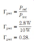
(26-19)
(26-20)

(26-21)
The voltage reflection coefficient (_) is found by taking the square root of the power reflection coefficient, so in this example it is equal to 0.529. These points are plotted at "A" and "B" in Fig. 26-5.
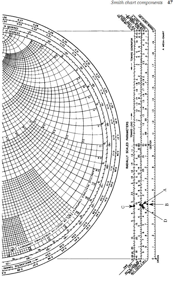
26-5 Radially scaled parameters.
Standing wave ratio (SWR) can be defined in terms of reflection coefficient:
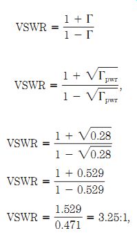
(26-22)
(26-23)
(26-24)
(26-25)
(26-26)

(26-27)
(26-28)
(26-29)
These points are plotted at "C" in Fig. 26-5. Shortly, you will work an example to show how these factors are calculated in a transmission-line problem from a known complex load impedance.
Transmission loss is a measure of the one-way loss of power in a transmission line because of reflection from the load.
Return loss represents the two-way loss so it is exactly twice the transmission loss. Return loss is found from:

(26-30)
(26-31)
(26-32)
This point is shown as "D" in Fig. 26-5. The transmission loss coefficient can be calculated from:
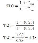
(26-33)
(26-34)
(26-35)
The TLC is a correction factor that is used to calculate the attenuation caused by mismatched impedance in a lossy, as opposed to the ideal "lossless," line. The TLC is found from laying out the impedance radius on the Loss Coefficient scale on the radially scaled parameters at the bottom of the chart.
Smith chart applications One of the best ways to demonstrate the usefulness of the Smith chart is by practical example. The following sections look at two general cases: transmission line problems and stub-matching systems.
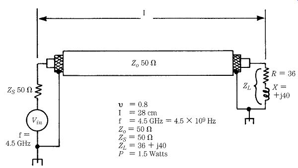
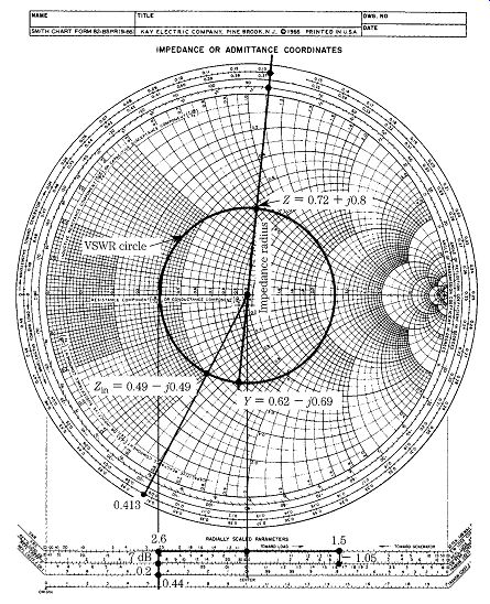
Transmission line problems Figure 26-6 shows a 50-ohm transmission line connected to a complex load impedance, ZL, of 36 _ j40 _. The transmission line has a velocity factor (v) of 0.80, which means that the wave propagates along the line at 8_10 the speed of light (c= 300,000,000 m/s). The length of the transmission line is 28 cm. The generator (Vin) is operated at a frequency of 4.5 GHz and produces a power output of 1.5 W. See what you can glean from the Smith chart (Fig. 26-7).
First, normalize the load impedance. This is done by dividing the load impedance by the systems impedance (in this case Z = 50-ohm ):
(26-36)
(26-37)
26-6 Transmission line and load circuit.
26-7 Solution to example.
The resistive component of impedance, Z, is located along the "0.72" pure resistance circle (see Fig. 26-7). Similarly, the reactive component of impedance Z is located by traversing the 0.72 constant resistance circle until the _j0.8 constant reactance circle is intersected. This point graphically represents the normalized load impedance Z _ 0.72 _ j0.80. A VSWR circle is constructed with an impedance radius equal to the line between "1.0" (in the center of the chart) and the "0.72 _ j0.8" point. At a frequency of 4.5 GHz, the length of a wave propagating in the transmission line, assuming a velocity factor of 0.80, is:

(26-38)
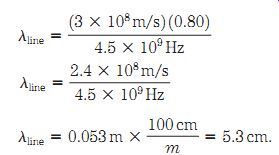
(26-39)
(26-40)
(26-41)
One wavelength is 5.3 cm, so a half-wavelength is 5.3 cm/2, or 2.65 cm. The 28-cm line is 28 cm/5.3 cm, or 5.28 wavelengths long. A line drawn from the center (1.0) to the load impedance is extended to the outer circle and it intersects the circle at 0.1325. Because one complete revolution around this circle represents one-half wavelength, 5.28 wavelengths from this point represents 10 revolutions plus 0.28 more. The residual 0.28 wavelengths is added to 0.1325 to form a value of (0.1325 _ 0.28) _ 0.413. The point "0.413" is located on the circle and is marked. A line is then drawn from 0.413 to the center of the circle and it intersects the VSWR circle at 0.49 _ j0.49, which represents the input impedance (Zin) looking into the line. To find the actual impedance represented by the normalized input impedance, you have to "de-normalize" the Smith chart impedance by multiplying the result by Z0:

(26-42)
(26-43)
This impedance must be matched at the generator by a conjugate matching net work. The admittance represented by the load impedance is the reciprocal of the load impedance and is found by extending the impedance radius through the center of the VSWR circle until it intersects the circle again. This point is found and represents the admittance Y = 0.62 - j0.69. Confirming the solution mathematically:
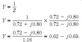
(26-44)
(26-45)
(26-46)
The VSWR is found by transferring the "impedance radius" of the VSWR circle to the radial scales. The radius (0.72 - 0.80) is laid out on the VSWR scale (topmost of the radially scaled parameters) with a pair of dividers from the center mark, and you find that the VSWR is approximately 2.6:1. The decibel form of VSWR is 8.3 dB (next scale down from VSWR) and this is confirmed by:

(26-47)
(26-48)
(26-49)
The transmission loss coefficient is found in a manner similar to the VSWR, using the radially scaled parameter scales. In practice, once you have found the VSWR, you need only drop a perpendicular line from the 2.6:1 VSWR line across the other scales.
In this case, the line intersects the voltage reflection coefficient at 0.44. The power reflection coefficient (Gpwr) is found from the scale and is equal to G2. The perpendicular line intersects the power reflection coefficient line at 0.20. The angle of reflection coefficient is found from the outer circles of the Smith chart. The line from the center to the load impedance (Z _ 0.72 _ j0.80) is extended to the Angle of Reflection Coefficient in Degrees circle and intersects it at approximately 84_. The reflection coefficient is therefore 0.44/84_. The transmission loss coefficient (TLC) is found from the radially scaled parameter scales also. In this case, the impedance radius is laid out on the Loss Coefficient scale, where it is found to be 1.5. This value is confirmed from:
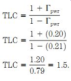
(26-50)
(26-51)
(26-52)
The Return Loss is also found by dropping the perpendicular from the VSWR point to the RET'N LOSS, dB line, and the value is found to be approximately 7 dB, which is confirmed by:

(26-53)
(26-54)
(26-55)
(26-56)
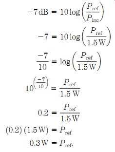
The reflection loss is the amount of RF power reflected back down the trans mission line from the load. The difference between incident power supplied by the generator (1.5 W, in this example), Pinc _ Pref _ Pabs, and the reflected power is the absorbed power (Pa) or, in the case of an antenna, the radiated power. The reflection loss is found graphically by dropping a perpendicular from the TLC point (or by laying out the impedance radius on the REFL. Loss, dB scale) and in this example (Fig. 26-7) is _1.05 dB. You can check the calculations: The return loss was _7 dB, so:
(26-57) (26-58) (26-59) (26-60) (26-61) (26-62) (26-63)
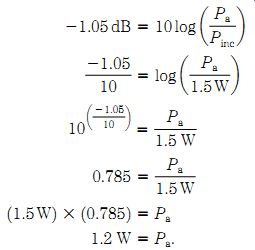
The power absorbed by the load (Pa) is the difference between incident power (Pinc) and reflected power (Pref). If 0.3 W is reflected, the absorbed power is (1.5 _ 0.3), or 1.2 W. The reflection loss is _1.05 dB and can be checked from:
(26-64) (26-65) (26-66) (26-67) (26-68) (26-69)
Now check what you have learned from the Smith chart. Recall that 1.5 W of 4.5-GHz microwave RF signal were input to a 50-ohm transmission line that was 28 cm long. The load connected to the transmission line has an impedance of 36 _ j40.
From the Smith chart:
Admittance (load): 0.62 - j0.69
VSWR: 2.6:1 VSWR (dB): 8.3 dB
Refl. coef. (E): 0.44
Refl. coef. (P): 0.2
Refl. coef. angle: 84_
Return loss: _7 dB
Refl. loss: _1.05 dB
Trans. loss. coef.: 1.5
Notice that in all cases, the mathematical interpretation corresponds to the graphical interpretation of the problem, within the limits of accuracy of the graphical method.
Stub matching systems
A properly designed matching system will provide a conjugate match to a complex impedance. Some sort of matching system or network is needed any time the load impedance (ZL) is not equal to the characteristic impedance (Zo) of the trans mission line. In a transmission-line system, it is possible to use a shorted stub connected in parallel with the line, at a critical distance back from the mismatched load, to affect a match. The stub is merely a section of transmission line that is shorted at the end not connected to the main transmission line. The reactance (hence also susceptance) of a shorted line can vary from __ to __, depending on length, so you can use a line of critical length L2 to cancel the reactive component of the load impedance. Because the stub is connected in parallel with the line, it is a bit easier to work with admittance parameters rather than impedance.
Consider the example of Fig. 26-8, in which the load impedance is Z _ 100 _ j60, which is normalized to 2.0 _ j1.2. This impedance is plotted on the Smith chart in Fig. 26-9 and a VSWR circle is constructed. The admittance is found on the chart at point Y _ 0.37 _ j0.22.
To provide a properly designed matching stub, you need to find two lengths. L1 is the length (relative to wavelength) from the load toward the generator (see L1 in Fig. 26-8); L2 is the length of the stub itself.
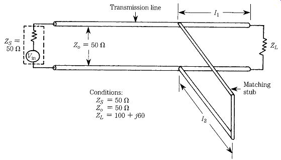
26-8 Matching stub length and position.
The first step in finding a solution to the problem is to find the points where the unit conductance line (1.0 at the chart center) intersects the VSWR circle; there are two such points shown in Fig. 26-9: 1.0 + j1.1 and 1.0 - j1.1. Select one of these (choose 1.0 _ j1.1) and extend a line from the center 1.0 point through the 1.0 + j1.1 point to the outer circle (WAVELENGTHS TOWARD GENERATOR). Similarly, a line is drawn from the center through the admittance point 0.37 - 0.22 to the outer cir cle. These two lines intersect the outer circle at the points 0.165 and 0.461. The distance of the stub back toward the generator is found from:

(26-70)
(26-71)
(26-72)
The next step is to find the length of the stub required. This is done by finding two points on the Smith chart. First, locate the point where admittance is infinite (far right side of the pure conductance line); second, locate the point where the admittance is 0 _ j1.1 (notice that the susceptance portion is the same as that found where the unit conductance circle crossed the VSWR circle). Because the conductance component of this new point is 0, the point will lie on the _j1.1 circle at the inter section with the outer circle. Now draw lines from the center of the chart through each of these points to the outer circle. These lines intersect the outer circle at 0.368 and 0.250. The length of the stub is found from:
(26-73)
(26-74)
From this analysis, you can see that the impedance, Z _ 100 _ j60, can be matched by placing a stub of a length 0.118_ at a distance 0.204_ back from the load.
The Smith chart in lossy circuits
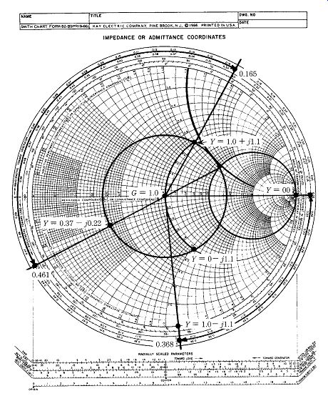
26-9 Solution to problem.
26-10 Solution.
Thus far, you have dealt with situations in which loss is either zero (i.e., ideal transmission lines) or so small as to be negligible. In situations where there is appreciable loss in the circuit or line, however, you see a slightly modified situation.
The VSWR circle, in that case, is actually a spiral, rather than a circle.
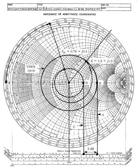
Figure 26-10 shows a typical situation. Assume that the transmission line is 0.60_ long and is connected to a normalized load impedance of Z _ 1.2 _ j1.2. An "ideal" VSWR circle is constructed on the impedance radius represented by 1.2 _ j1.2. A line ("A") is drawn, from the point where this circle intersects the pure resistance baseline ("B"), perpendicularly to the ATTEN 1 dB/MAJ. DIV. line on the radially scaled parameters. A distance representing the loss (3 dB) is stepped off on this scale. A second perpendicular line is drawn from the _3-dB point back to the pure resistance line ("C"). The point where "C" intersects the pure resistance line be comes the radius for a new circle that contains the actual input impedance of the line. The length of the line is 0.60 , so you must step back (0.60 _ 0.50)_ or 0.1_.
This point is located on the outer circle. A line is drawn from this point to the 1.0 center point. The point where this new line intersects the new circle is the actual input impedance (Zin). The inter section occurs at 0.76 _ j0.4, which (when de-normalized) represents an input impedance of 38 _ j20 _.
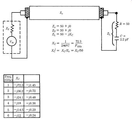
26-11 Load and source-impedance transmission-line circuit.
Frequency on the Smith chart
A complex network may contain resistive, inductive reactance, and capacitive reactance components. Because the reactance component of such impedances is a function of frequency, the network or component tends to also be frequency sensitive. You can use the Smith chart to plot the performance of such a network with respect to various frequencies. Consider the load impedance connected to a 50-ohm transmission line in Fig. 26-11. In this case, the resistance is in series with a 2.2-pF capacitor, which will exhibit a different reactance at each frequency. The impedance of this network is:
(26-75)
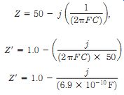
(26-76)
(26-77)
(26-78)
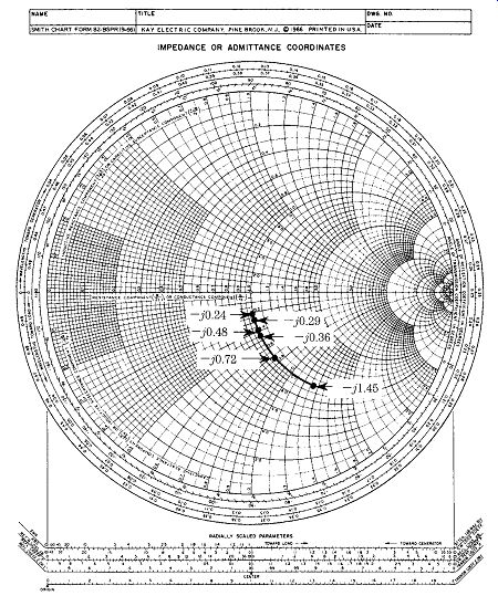
26-12 Plotted points.

(26-79)
(26-80)
The normalized impedances for the sweep of frequencies from 1 to 6 GHz are therefore:

(26-81)
(26-82)
(26-83) (26-84) (26-85) (26-86)
These points are plotted on the Smith chart in Fig. 26-12. For complex net works, in which both inductive and capacitive reactance exist, take the difference between the two reactances (i.e., X= XL - XC).