AMAZON multi-meters discounts AMAZON oscilloscope discounts
Fixed capacitors
Several types of fixed capacitors are used in typical electronic circuits. They are classified by dielectric type: paper, mylar, ceramic, mica, polyester, and others.
The construction of an old-fashioned paper capacitor is shown in FIG. 14. It consists of two strips of metal foil sandwiched on both sides of a strip of paraffin wax paper. The strip sandwich is then rolled up into a tight cylinder. This rolled up cylinder is then packaged in either a hard plastic, bakelite, or paper-and wax case. When the case is cracked, or the wax plugs are loose, replace the capacitor even though it tests as good-it won't be for long. Paper capacitors come in values from about 300 pF to about 4 uF. The breakdown voltages will be from 100 to 600 WVdc.
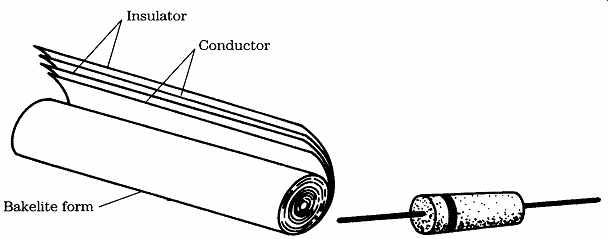
FIG. 14 Paper capacitor construction.
The paper capacitor was used for a number of different applications in older circuits, such as bypassing, coupling, and dc blocking. Unfortunately, no component is perfect. The long rolls of foil used in the paper capacitor exhibit a significant amount of stray inductance. As a result, the paper capacitor is not used for high frequencies.
Although they are found in some shortwave receiver circuits, they are rarely (if ever) used at VHF.
In modern applications, or when servicing older equipment containing paper capacitors, use a mylar dielectric capacitor in place of the paper capacitor. Select a unit with exactly the same capacitance rating and a WVdc rating that is equal to or greater than the original WVdc rating.
Several different forms of ceramic capacitors are shown in FIG. 15. These capacitors come in values from a few picofarads to 0.5 uF. The working voltages range from 400 WVdc to more than 30,000 WVdc. The common garden-variety disk ceramic capacitors are usually rated at either 600 to 1000 WVdc. Tubular ceramic capacitors are typically much smaller in value than disk or flat capacitors and are used extensively in VHF and UHF circuits for blocking, decoupling, bypassing, coupling, and tuning.
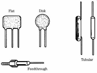
FIG. 15 Ceramic capacitors.
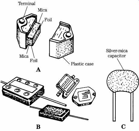
FIG. 16 Mica capacitors.
The feedthrough type of ceramic capacitor is used to pass dc and low-frequency ac lines through a shielded panel. These capacitors are often used to filter or decouple lines that run between circuits separated by the shield for purposes of electro magnetic interference (EMI) reduction.
Ceramic capacitors are often rated as to the temperature coefficient. This specification is the change of capacitance per change in temperature in degrees Celsius.
A "P" prefix indicates a positive temperature coefficient, an "N" indicates a negative temperature coefficient, and the letters "NPO" indicate a zero temperature coefficient (NPO stands for "negative positive zero"). Do not ad lib on these ratings when servicing a piece of electronic equipment. Use exactly the same temperature coefficient as the original manufacturer used. Nonzero temperature coefficients are often used in oscillator circuits to temperature compensate the oscillator's frequency drift.
Several different types of mica capacitors are shown in FIG. 16. The fixed mica capacitor consists of metal plates on either side of a sheet of mica or a sheet of mica silvered with a deposit of metal on either side. The range of values for mica capacitors tends to be 50 pF to 0.02 uF at voltages in the range of 400 to 1000 WVdc. The mica capacitor shown in FIG. 16C is called a silver mica capacitor. These capacitors have a low temperature coefficient, although for most applications, an NPO disk ceramic capacitor will provide better service than all but the best silver mica units (silver mica temperature coefficients have greater variation than NPO temperature coefficients). Mica capacitors are typically used for tuning and other uses in higher frequency applications.
Today's equipment designer has a number of different dielectric capacitors avail able that were not commonly available (or available at all) a few years ago. Polycarbonate, polyester, and polyethylene capacitors are used in a wide variety of applications where the capacitors described in the previous paragraphs once ruled supreme. In digital circuits, tiny 100-WVdc capacitors carry ratings of 0.01 to 0.5 uF.
These are used for decoupling the noise on the +/- 5-Vdc power-supply line. In circuits, such as timers and op-amp Miller integrators, where the leakage resistance across the capacitor becomes terribly important, it might be better to use a poly ethylene capacitor.
Check current catalogs for various old and new capacitor styles. The applications paragraph in the catalog will tell you what applications each can be used for as well as provide a guide to the type of antique capacitor it will replace.
Capacitors in ac circuits
When an electrical potential is applied across a capacitor, current will flow as charge is stored in the capacitor. As the charge in the capacitor increases, the volt age across the capacitor plates rises until it equals the applied potential. At this point, the capacitor is fully charged, and no further current will flow.
FIG. 17 shows an analogy for the capacitor in an ac circuit. The actual circuit is shown in FIG. 17A. It consists of an ac source connected in parallel across the capacitor. The mechanical analogy is shown in FIG. 17B. The capacitor consists of a two-chambered cylinder in which the upper and lower chambers are separated by a flexible membrane or diaphragm. The wires are pipes to the ac source (which is a pump). As the pump moves up and down, pressure is applied to the first side of the diaphragm and then the other, alternately forcing fluid to flow into and out of the two chambers of the capacitor.
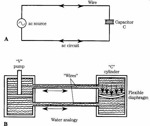
FIG. 17 Capacitor circuit analogy and capacitor circuit action.
The ac circuit mechanical analogy is not perfect, but it works for these purposes.
Apply these ideas to the electrical case. FIG. 17 shows a capacitor connected across an ac (sine-wave) source. In FIG. 17A, the ac source is positive, so negatively charged electrons are attached from plate A to the ac source and electrons from the negative terminal of the source are repelled toward plate B of the capacitor.
On the alternate half-cycle ( FIG. 17B), the polarity is reversed. Electrons from the new negative pole of the source are repelled toward plate A of the capacitor and electrons from plate B are attracted toward the source. Thus, current will flow in and out of the capacitor on alternating half-cycles of the ac source.
Voltage and current in capacitor circuits
Consider the circuit in FIG. 18: an ac source connected in parallel with the capacitor. It is the nature of a capacitor to oppose these changes in the applied voltage (the inverse of the action of an inductor). As a result, the voltage lags behind the current by 90 degrees. These relationships are shown in terms of sine waves in Fig.
FIG. 18B and in vector form in FIG. 18C.
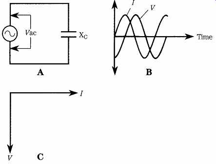
FIG. 18 (A) Ac circuit using a capacitor; (B) sine-wave relationship between
V and I; (C) vector representation.
Do you remember the differences in the actions of inductors and capacitors on voltage and current? In earlier texts, the letter E was used to denote voltage, so you could make a little mnemonic: "ELI the ICE man." "ELI the ICE man" suggests that in the inductive (L) circuit, the voltage (E) comes before the current (I): ELI; in a capacitive (C) circuit, the current comes be fore the voltage: ICE.
The action of a circuit containing a resistance and capacitance is shown in Fig. 219A. As in the case of the inductive circuit, there is no phase shift across the resistor, so the R vector points in the east direction ( FIG. 19B). The voltage across the capacitor, however, is phase-shifted 90 so its vector points south. The total resultant phase shift () is found using the Pythagorean rule to calculate the angle between VR and VT.
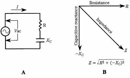
FIG. 19 (A) Resistor-capacitor (RC) circuit; (B) vector representation
of circuit action.
The impedance of an RC circuit is found in exactly the same manner as the impedance of an RL circuit; that is, as the root of the sum of the squares:
(Eqn. 19)
LC Resonant tank circuits
When you use an inductor and a capacitor together in the same circuit, the combination forms an LC resonant circuit, which is sometimes called a tank circuit or resonant tank circuit. These circuits can be used to tune a radio receiver as well as in other applications. There are two basic forms of LC resonant tank circuit: series ( FIG. 20A) and parallel ( FIG. 20B). These circuits have much in common and much that makes them fundamentally different from each other.
The condition of resonance occurs when the capacitive reactance and inductive reactance are equal. As a result, the resonant tank circuit shows up as purely resistive at the resonant frequency (see FIG. 20C) and as a complex impedance at other frequencies. The LC resonant tank circuit operates by an oscillatory exchange of energy between the magnetic field of the inductor and the electrostatic field of the capacitor, with a current between them carrying the charge.
Because the two reactances are both frequency-dependent, and because they are inverse to each other, the resonance occurs at only one frequency (FR). You can calculate the standard resonance frequency by setting the two reactances equal to each other and solving for F. The result is as follows:
(Eqn. 20)
where
F is in hertz (Hz)
L is in henrys (H)
C is in farads (F).
Series-resonant circuits
The series-resonant circuit ( FIG. 20A), like other series circuits, is arranged so that the terminal current (I) from the source (V) flows in both components equally.
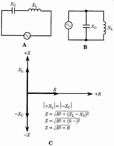
FIG. 20 (A) Series inductor-capacitor (LC) circuit; (B) parallel LC circuit;
(C) vector relationships.
The vector diagrams of FIG. 21A through 2-21C show the situation under three different conditions:
• FIG. 21A: The inductive reactance is larger than the capacitive reactance, so the excitation frequency is greater than FR. Notice that the voltage drop across the inductor is greater than that across the capacitor, so the total circuit looks like it contains a small inductive reactance.
• FIG. 21B: The situation is reversed. The excitation frequency is less than the resonant frequency, so the circuit looks slightly capacitive to the outside world.
• FIG. 21C: The excitation frequency is at the resonant frequency, so XC _ XL and the voltage drops across the two components are of equal but opposite phase.
In a circuit that contains a resistance, an inductive reactance, and a capacitive reactance, there are three vectors (XL, XC, and R) to consider ( FIG. 22) plus a resultant vector. As in the other circuit, the north direction is XL, the south direction is XC, and the east direction is R. Using the parallelogram method, construct a resultant for R and XC, which is shown as vector A. Next, construct the same kind of vector (B) for R and XL. The resultant vector (C) is made using the parallelogram method on vectors A and B. Vector C represents the impedance of the circuit: The magnitude is represented by the length and the phase angle by the angle between vector C and R.
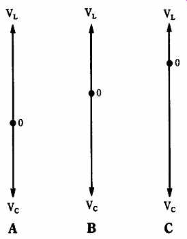
FIG. 21 Vector relationships for circuits in which (A) XL > XC; (B) XL
< XC; and (C) XL = XC.
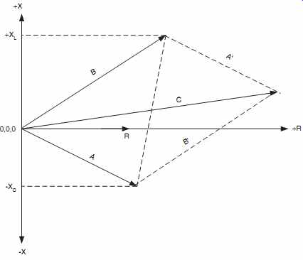
FIG. 22 Vector relationships for an RLC circuit.
FIG. 23A shows a series-resonant LC tank circuit, and FIG. 23B shows the current and impedance as a function of frequency. Series-resonant circuits have a low impedance at the resonant frequency and a high impedance at all other frequencies. As a result, the line current from the source is maximum at the resonant frequency and the voltage across the source is minimum.
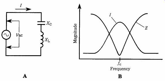
FIG. 23 (A) Series-resonant LC circuit; (B) I and Z vs frequency response.
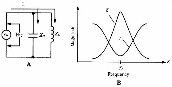
FIG. 24 (A) Parallel-resonant LC circuit; (B) I and Z vs frequency response.
Parallel-resonant circuits
The parallel-resonant tank circuit ( FIG. 24A) is the inverse of the series resonant circuit. The line current from the source splits and flows separately in the inductor and capacitor.
The parallel-resonant circuit has its highest impedance at the resonant frequency and a low impedance at all other frequencies. Thus, the line current from the source is minimum at the resonant frequency ( FIG. 24B) and the voltage across the LC tank circuit is maximum. This fact is important in radio tuning circuits, as you will see later.
Choosing component values for LC-resonant tank circuits
In some cases, one of the two basic type of resonant tank circuit (either series or parallel) is clearly preferred over the other, but in other cases either could be used if it is used correctly. For example, in a wave trap (i.e., a circuit that prevents a particular frequency from passing) a parallel-resonant circuit in series with the signal line will block its resonant frequency while passing all frequencies removed from resonance; a series-resonant circuit shunted across the signal path will bypass its resonant frequency to common (or "ground") while allowing frequencies removed from resonance to pass.
LC-resonant tank circuits are used to tune radio receivers; it is these circuits that select the station to be received while rejecting others. A superheterodyne radio receiver (the most common type) is shown in simplified form in FIG. 25. According to the superhet principal, the radio frequency being received (FRF) is converted to another frequency, called the intermediate frequency (FIF) by being mixed with a local oscillator signal (FLO) in a nonlinear mixer stage. The output of the untamed mixer would be a collection of frequencies defined by the following:
FIF = mFRF +/- nFLO (Eqn. 21)
where m and n are either integers or zero. For the simplified case that is the subject of this section only the first pair of products (m= n = 1) are considered, so the out put spectrum will consist of FRF, FLO, FRF = FLO (difference frequency), and FRF - FLO (sum frequency). In older radios, for practical reasons, the difference frequency was selected for FIF, today either sum or difference frequencies can be selected, de pending on the design of the radio.
Several LC tank circuits are present in this notional superhet radio. The antenna tank circuit (C1/L1) is found at the input of the RF amplifier stage, or if no RF amplifier is used it is at the input to the mixer stage. A second tank circuit (L2/C2), tuning the same range as L1/C1, is found at the output of the RF amplifier or at the input of the mixer. Another LC tank circuit (L3/C3) is used to tune the local oscillator; it is this tank circuit that sets the frequency that the radio will receive.
Additional tank circuits (only two shown) can be found in the IF amplifier section of the radio. These tank circuits will be fixed-tuned to the IF frequency, which in common AM broadcast-band (BCB) radio receivers is typically 450, 455, 460, or 470 kHz depending on the designer's choices (and sometimes country of origin).
Other IF frequencies are also used, but these are most common. FM broadcast receivers typically use a 10.7-MHz IF, and shortwave receivers might use a 1.65-, 8.83-, or 9-MHz frequency or an IF frequency above 30 MHz.
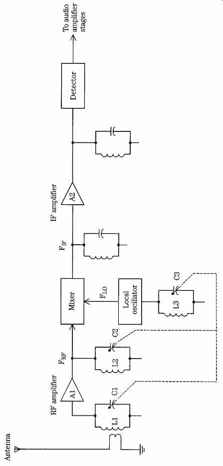
FIG. 25 Parallel-resonant circuits used in a radio receiver.
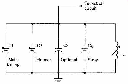
FIG. 26 Capacitors used in a typical radio tuning circuit.
The tracking problem
On a radio that tunes the front end with a single knob, which is the case in al most all receivers today, the three capacitors (C1 through C3 in FIG. 26) are typically ganged (i.e., mounted on a single rotor shaft). These three tank circuits must track each other; that is, when the RF amplifier is tuned to a certain radio signal frequency, the LO must produce a signal that is different from the RF frequency by the amount of the IF frequency. Perfect tracking is rare, but the fact that your single knob-tuned radio works is testimony to the fact that the tracking is not too terrible.
The issue of tracking LC tank circuits for the AM BCB receiver has not been a major problem for many years: the band limits are fixed over most of the world and, component manufacturers offer standard adjustable inductors and variable capacitors to tune the RF and LO frequencies. Indeed, some even offer three sets of coils: antenna, mixer input/RF amp output, and LO. The reason why the antenna and mixer/RF coils are not the same, despite tuning to the same frequency range, is that these locations see different distributed or "stray" capacitances. In the United States, it is standard to use a 10- to 365-pF capacitor and a 220-uH inductor for the 540- to 1700-kHz AM BCB. In other countries, slightly different combinations are used; for example, 320, 380, 440, and 500 pF and others are seen in catalogs.
Recently, however, two events coincided that caused me to examine the method of selecting capacitance and inductance values. First, I embarked on a design project to produce an AM DX-er's receiver that had outstanding performance characteristics. Second, the AM broadcast band was recently extended so that the upper limit is now 1700 rather than 1600 kHz. The new 540- to 1700-kHz band is not accommodated by the now-obsolete "standard" values of inductance and capacitance. So I calculated new candidate values.
The RF amplifier/antenna tuner problem
In a typical RF tank circuit, the inductance is kept fixed (except for a small adjustment range that is used for overcoming tolerance deviations) and the capacitance is varied across the range. The frequency changes as the square root of the capacitance changes. If F1 is the minimum frequency in the range and F2 is the maximum frequency then the relationship is as follows:
(Eqn. 22)
or, in a rearranged form that some find more applicable:
(Eqn. 23)
In the case of the new AM receiver, I wanted an overlap of about 15 kHz at the bottom end of the band and 10 kHz at the upper end and so needed a resonant tank circuit that would tune from 525 to 1710 kHz. In addition, because variable capacitors are widely available in certain values based on the old standards, I wanted to use a "standard" AM BCB variable capacitor. A 10- to 380-pF unit from a U.S. vendor was selected.
The minimum required capacitance, Cmin, can be calculated from the following:
(Eqn. 24)
where
F1 is the minimum frequency tuned
F2 is the maximum frequency tuned
Cmin is the minimum required capacitance at F2
ΔC is the difference between Cmax and Cmin.
Example
Find the minimum capacitance needed to tune 1710 kHz when a 10- to 380-pF capacitor (ΔC = 380 - 10 pF = 370 pF) is used and the minimum frequency is 525 kHz.
Solution
The maximum capacitance must be Cmin + ΔC or 38.51 + 370 pF = 408.51 pF.
Because the tuning capacitor (C1 in FIG. 26) does not have exactly this range, external capacitors must be used and because the required value is higher than the normal value additional capacitors are added to the circuit in parallel to C1. Indeed, because somewhat unpredictable "stray" capacitances also exist in the circuit, the tuning capacitor values should be a little less than the required values in order to accommodate strays plus tolerances in the actual (versus published) values of the capacitors. In FIG. 26, the main tuning capacitor is C1 (10 to 380 pF), C2 is a small value trimmer capacitor used to compensate for discrepancies, C3 is an optional capacitor that might be needed to increase the total capacitance, and Cs is the stray capacitance in the circuit.
The value of the stray capacitance can be quite high-especially if other capacitors in the circuit are not directly used to select the frequency (e.g., in Colpitts and Clapp oscillators, the feedback capacitors affect the LC tank circuit). In the circuit that I was using, however, the LC tank circuit is not affected by other capacitors. Only the wiring strays and the input capacitance of the RF amplifier or mixer stage need be accounted. From experience, I apportioned 7 pF to Cs as a trial value.
The minimum capacitance calculated was 38.51; there is a nominal 7 pF of stray capacitance and the minimum available capacitance from C1 is 10 pF. Therefore, the combined values of C2 and C3 must be 38.51 pF - 10 pF - 7 pF, or 21.5 pF. Because there is considerable reasonable doubt about the actual value of Cs, and because of tolerances in the manufacture of the main tuning variable capacitor (C1), a wide range of capacitance for C2 + C3 is preferred. It is noted from several catalogs that 21.5 pF is near the center of the range of 45- and 50-pF trimmer capacitors. For ex ample, one model lists its range as 6.8 to 50 pF; its center point is only slightly re moved from the actual desired capacitance. Thus, a 6.8- to 50-pF trimmer was selected, and C3 was not used.
Selecting the inductance is a matter of choosing the frequency and associated required capacitance at one end of the range and calculating from the standard resonance equation solved for L:
The RF amplifier input LC tank circuit and the RF amplifier output LC tank circuit are slightly different cases because the stray capacitances are somewhat different. In the example, I am assuming a JFET transistor RF amplifier, and it has an input capacitance of only a few picofarads. The output capacitance is not a critical issue in this specific case because I intend to use a 1-mH RF choke in order to pre vent JFET oscillation. In the final receiver, the RF amplifier can be deleted altogether, and the LC tank circuit described will drive a mixer input through a link-coupling circuit.
The local oscillator (LO) problem
The local oscillator circuit must track the RF amplifier and must also tune a frequency range that is different from the RF range by the amount of the IF frequency (455 kHz). In keeping with common practice, I selected to place the LO frequency 455 kHz above the RF frequency. Thus, the LO must tune the range from 980 to 2165 kHz.
Three methods can be used to make the local oscillator track with the RF amplifier frequency when single-shaft tuning is desired: the trimmer capacitor method, the padder capacitor method, and the different-value cut-plate capacitor method.
Trimmer capacitor method
The trimmer capacitor method is shown in FIG. 27 and is the same as the RF LC tank circuit. Using exactly the same method as before, a frequency ratio of 2165/980 yields a capacitance ratio of (2165/980)2 _ 4.88:1. The results are a minimum capacitance of 95.36 pF and a maximum capacitance of 465.36 pF. An inductance of 56.7 uH is needed to resonate these capacitances to the LO range.
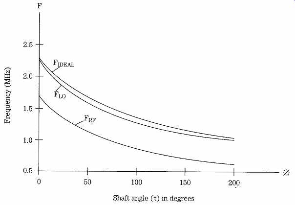
FIG. 27 The tracking problem.
There is always a problem associated with using the same identical capacitor for both RF and LO. It seems that there is just enough difference that tracking between them is always a bit off. FIG. 27 shows the ideal LO frequency and the calculated LO frequency. The difference between these two curves is the degree of non-tracking. The curves overlap at the ends but are awful in the middle. There are two cures for this problem. First, use a padder capacitor in series with the main tuning capacitor ( FIG. 28). Second, use a different-value cut-plate capacitor.
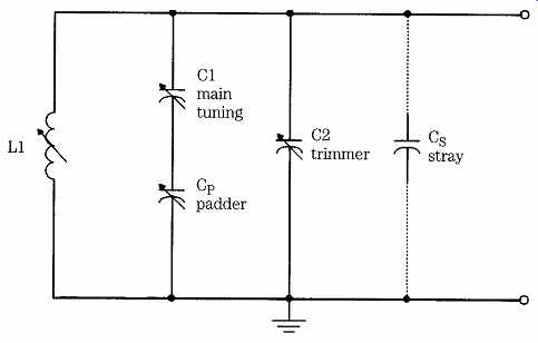
FIG. 28 Oscillator-tuned circuit using padder capacitor.
FIG. 28 shows the use of a padder capacitor (Cp) to change the range of the LO section of the variable capacitor. This method is used when both sections of the variable capacitor are identical. Once the reduced capacitance values of the C1/Cp combination are determined, the procedure is identical to that above. But first, you must calculate the value of the padder capacitor and the resultant range of the C1/Cp combination. The padder value is calculated from the following:
(Eqn. 25)
which solves for Cp. For the values of the selected main tuning capacitor and LO:
1max p 1 1min p
(Eqn. 26)
Solving for Cp by the least common denominator method (crude, but it works) yields a padder capacitance of 44.52 pF. The series combination of 44.52 pF and a 10- to 380-pF variable yields a range of 8.2 to 39.85 pF. An inductance of 661.85 pF is needed for this capacitance to resonate over 980 to 2165 kHz.
Tuned RF/IF transformers
Most of the resonant circuits used in radio receivers are actually tuned RF transformers that couple signal from one stage to another. FIG. 29 shows several popular forms of tuned, or coupled, RF/IF tank circuits. In FIG. 29A, one winding is tuned and the other is untuned. In the configurations shown, the untuned winding is the secondary of the transformer. This type of circuit is often used in transistor and other solid-state circuits or when the transformer has to drive either a crystal or mechanical bandpass filter circuit. In the reverse configuration (L1 _ output, L2 _ input), the same circuit is used for the antenna coupling network or as the interstage transformer between RF amplifiers in TRF radios.
The circuit in FIG. 29B is a parallel-resonant LC tank circuit that is equipped with a low-impedance tap. This type of circuit is used to drive a crystal detector or other low-impedance load. Another circuit for driving a low-impedance load is shown in FIG. 29C. This circuit splits the capacitance that resonates the coil into two series capacitors. As a result, it is a capacitive voltage divider. The circuit in FIG. 29D uses a tapped inductor for matching low-impedance sources (e.g., antenna circuits) and a tapped capacitive voltage divider for low-impedance loads. Finally, the circuit in FIG. 29E uses a tapped primary and tapped secondary winding in order to match two low-impedance loads while retaining the sharp bandpass characteristics of the tank circuit.
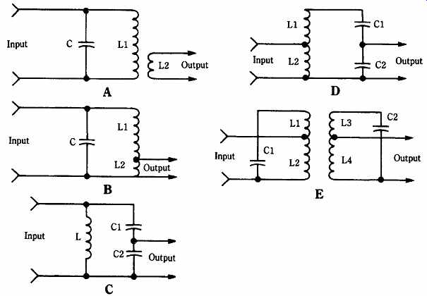
FIG. 29 Coupling circuits used in radio receivers and transmitters.
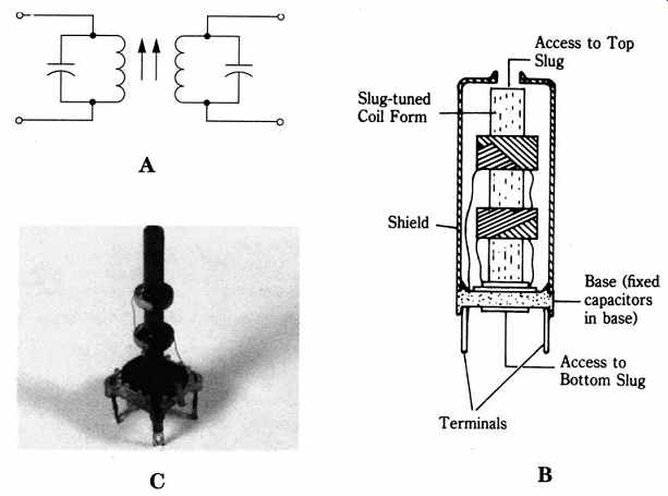
FIG. 30 (A) Tuned RF or IF transformer; (B) IF/RF transformer construction;
(C) actual transformer.
Construction of RF/IF transformers
The tuned RF/IF transformers built for radio receivers are typically wound on a common cylindrical form and surrounded by a metal shield that can prevent inter action of the fields of coils that are in close proximity to each other. FIG. 30A shows the schematic for a typical RF/IF transformer, and the sectioned view ( FIG. 30B) shows one form of construction. This method of building transformers was common at the beginning of World War II and continued into the early transistor era. The capacitors were built into the base of the transformer, and the tuning slugs were accessed from holes in the top and bottom of the assembly. In general, expect to find the secondary at the bottom hole and the primary at the top holes.
The term universal wound refers to a cross-winding system that minimizes the interwinding capacitance of the inductor and raises the self-resonant frequency of the inductor (a good thing). An actual example of an RF/IF transformer is shown in FIG. 30C. The smaller type tends to be post-WWII, and the larger type is pre-WWII.
Bandwidth of RF/IF transformers
FIG. 31A shows a parallel-resonant RF/IF transformer, and FIG. 31B shows the usual construction in which the two coils (L1 and L2) are wound at distance d apart on a common cylindrical form. The bandwidth of the RF/IF transformer is the difference between the frequencies where the signal voltage across the output winding falls off 6 dB from the value at the resonant frequency (FR), as shown in FIG. 31C. If F1 and F2 are 6-dB (also called the 3-dB point when signal power is measured instead of voltage) frequencies, then the bandwidth is F2 _ F1. The shape of the frequency response curve in FIG. 31C is said to represent critical coupling.
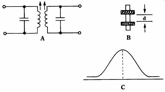
FIG. 31 Moderate coupling IF transformer. (A) The circuit; (B) coil spacing;
(C) bandpass response.
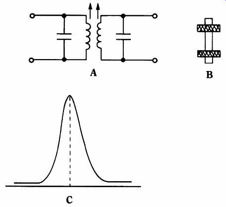
FIG. 32 Loose coupling IF transformer. (A) The circuit; (B) coil spacing;
(C) bandpass response.
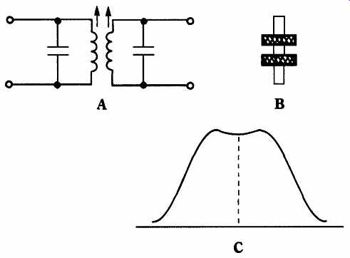
FIG. 33 Over-critical coupling IF transformer. (A) The circuit; (B) coil
spacing; (C) bandpass response.
An example of a subcritical or under-coupled RF/IF transformer is shown in FIG. 32. As shown in Figs. 2-32A and 2-32B, the windings are farther apart than in the critically coupled case, so the bandwidth ( FIG. 32C) is much narrower than in the critically coupled case. The sub-critically coupled RF/IF transformer is often used in shortwave or communications receivers in order to allow the narrow band width to discriminate between adjacent channels.
The overcritically coupled RF/IF transformer is shown in FIG. 33. Notice in Figs. 33A and 33B that the windings are closer together, so the bandwidth ( FIG. 33C) is much broader. In some radio schematics and service manuals (not to mention early textbooks), this form of coupling was sometimes called high-fidelity coupling because it allowed more of the sidebands of the signal (which carry the audio modulation) to pass with less distortion of frequency response.
The bandwidth of the resonant tank circuit, or the RF/IF transformer, can be summarized in a figure of merit called Q. The Q of the circuit is the ratio of the band width to the resonant frequency as follows: Q_BW/FR. An overcritically coupled circuit has a low Q, while a narrow bandwidth subcritically coupled circuit has a high Q.
A resistance in the LC tank circuit will cause it to broaden; that is, to lower its Q.
The loaded Q (i.e., Q when a resistance is present, as in FIG. 34A) is always less than the unloaded Q. Some radios use a switched resistor ( FIG. 34B) to allow the user to broaden or narrow the bandwidth. This switch might be labeled fidelity or tone or something similar on radio receivers.
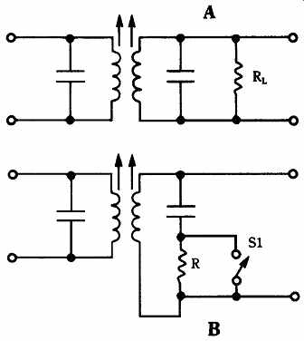
FIG. 34 Resistor loading to broaden response. (A) Parallel method; (B)
hi-fi switch.
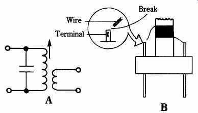
FIG. 35 (A) IF transformer circuit; (B) typical defect.
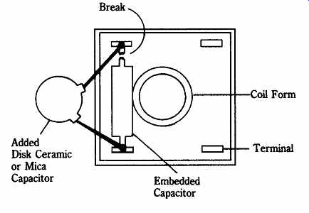
FIG. 36 Replacement of the embedded capacitor with a disk ceramic or silvered
mica fixed capacitor.
Problems with RF/IF transformers
The IF and RF transformers represent a high potential for intermittent problems in radio receivers. There are two basic forms of problems with the IF transformer: intermittent operation and intermittent noise. The best cure for a bad IF or RF transformer is replacement, but because old IF and RF transformers are not always available today, more emphasis must be placed on repair of the transformer.
FIG. 35A shows the basic circuit for a single-tuned IF transformer (others might have a tuned secondary winding). If one of the very-fine wires making up the coil breaks ( FIG. 35B), then operation is interrupted. The problem can usually be diagnosed by lightly tapping on the shield can of the transformer or by using a signal tracer or signal generator to find where the signal is interrupted. In some cases, the plate voltage of the IF amplifier is interrupted when the transformer opens. This can be spotted using a dc voltmeter.
Repairing the IF transformer is a delicate operation. Examine the shield to determine how it is assembled. If it is secured with a screw or nut, simply remove the screw (or nut). If the IF transformer is sealed by metal tabs, then you must very carefully pry the tabs open (do not break them or bend them too far). Slide the base and coil assembly out of the shield. If there is enough slack on the broken wire, simply solder the wire back onto the terminal. The heat of the soldering iron tip will burn away the enamel insulation. If the wire does not have enough slack, then add a little length to the terminal by soldering a short piece of solid wire to the terminal and then solder the IF transformer wire to the added wire. In some cases, it is possible to remove a portion of one turn of the transformer winding in order to gain extra length, but this procedure will change the tuning.
A noisy IF transformer needs replacement, but the problem is the lack of original or replacement components. The capacitor can be replaced on many IF trans formers. If the capacitor is a discrete component soldered to the base, it is simple to replace it with another similar (if not identical) capacitor. But if the IF transformer uses an embedded mica capacitor (FIG. 36), then the job becomes more complex.
If the capacitor element is visible (as in FIG. 36), then clip one end of the capacitor where it is attached to the terminal. Bridge a disk ceramic or mica capacitor between the two terminals. The value of the capacitor must be found experimentally--it is the value that will resonate the coil to the IF.
If the capacitor is embedded and not visible, it might become necessary to install a new terminal and solder the added capacitor to that terminal (with appropriate external circuit modifications).